
SPLITTING FACTS USING WEIGHTS
Liga Grundmane, Laila Niedrite
University of Latvia, Department of Computer Science,
19 Raina blvd., Riga, Latvia
Keywords: Data Warehouse, Weights, Fact Granularity.
Abstract: A typical data warehouse report is the dynamic representation of some objects’ behaviour or changes of
objects’ properties.
If this behaviour is changing, it is difficult to make such reports in an easy way. It is
possible to use the fact splitting to make this task simpler and more comprehensible for users. In the
presented paper two solutions of splitting facts by using weights are described. One of the possible solutions
is to make the proportional weighting accordingly to splitted record set size. It is possible to take into
account the length of the fact validity time period and the validity time for each splitted fact record.
1 INTRODUCTION
Following the classical data warehouse theory
(Kimball, 1996), (Inmon, 1996) there are fact tables
and dimension tables in the data warehouse.
Measures about the objects of interest of business
analysts are stored in the fact table. This information
is usually represented as different numbers. At the
same time the information about properties of these
objects is stored in the dimensions.
A typical data warehouse report is a dynamic
representation of some objects’ behavior. If this
behavior is changing slowly, we can say the fact is
slowly evolving. It is difficult to make such reports
in an easy way. Therefore we have introduced fact
splitting using weights. This method gives a
possibility to solve the problem.
To describe slowly evolving fact we can say that
the fact has a value for a time period and following
this is a situation when the given fact corresponds to
many time units in the time dimension.
In some sources some situations are described
when one object has a set of properties or it is
connected with a set of other objects. This set can be
considered as one entirety. To specify the percentage
for each member of the set, weights are used. Such
situation usually is called “many to many”
relationship between the dimension table and the
fact table. To cope with these situations, the bridge
tables are introduced. Each member from the set
that is defined in the bridge table, gets its weight.
Summarized total of weights for all members from
one set have to be 100 percent. There exists an
opinion that bridge tables are not easily
understandable for users, however such a modeling
technique satisfies business requirements quite good.
If a data mart exists with only aggregated values,
it is not possible to get the exact initial values. It is
possible to get only some approximation. So if we
need to lower the fact table grain, we have to split
the aggregated fact value accordingly to the chosen
granularity.
In section 2 related work is presented. Section 3
gives data warehouse related definitions. Splitting
fact using weights is introduced in section 4. It is
followed by an example in section 5. Section 6
concludes the paper and points out some further
research directions.
2 RELATED WORK
The concept of “slowly evolving fact” was
introduced by Chen, (Cochinwala, and Yueh, 1999).
The authors argue that in some cases the classical
approach to keep measurable facts in the star schema
is not the best solution. If the fact value remains
unchanged during some time period, the redundant
values of measures, being at the same time the
snapshots of the fact in every particular time unit
during the period, are stored in the fact table. Instead
of that a “transaction-oriented” fact table could be
used, where the fact table records represent
transaction by structure with measured fact value
253
Grundmane L. and Niedrite L. (2006).
SPLITTING FACTS USING WEIGHTS.
In Proceedings of the Eighth International Conference on Enterprise Information Systems - DISI, pages 253-258
DOI: 10.5220/0002447402530258
Copyright
c
SciTePress

and transaction start and end time representing the
time period with unchanged fact value and very
likely with long duration.
The real transaction-level fact tables with facts
that represent transactions in data sources are
discussed in (Kimball, 1996). (Chen, Cochinwala,
and Yueh, 1999) use the “transaction-oriented” fact
table for answering the questions concerning the
artificial transaction itself, e.g. the average length of
the transaction duration, but in cases when lower
detail data is necessary, a virtual cube is created to
answer the question.
The dimension tables are usually associated with
the fact table using the relationship “one to many”.
The real data warehouse projects sometime request
the solutions for “many to many” situations keeping
unchanged the star schema structure and also the
simplicity of the model. (Song et al., 2001) describes
different solutions for “many to many” relationship.
Two of them are connected with lowering the grain
of the fact table. When fact values are not accessible
they are precomputed and divided according
weights. Authors consider the solutions for
transaction fact tables.
The most popular solution for “many to many”
relationship between the fact and dimension tables is
known from Kimball’s books (Kimball et.al., 1998),
(Kimball and Ross, 2002), where the solution with
the bridge tables is explained. The attribute groups
are defined in the bridge table from attributes of the
dimension table and the weighting factors are
assigned for each attribute within the group.
(Kimball and Ross, 2002) mention also the possible
change of the granularity of the fact table, where the
detailed fact value could be computed from given
fact value multiplied with the weighting factors for
each attribute within the corresponding attribute
group from the bridge table. The result is the
growing number of the fact table records after this
activity. The solution could turn into a problem as
well in the case when more than one dimension have
“many to many” relationships with the fact table,
because the explicit meaning of the newly computed
fact is not possible to define.
(Eder, Koncilia, and Kogler, 2002) suggest the
solution with temporal data warehouse to depict the
structural changes. The dimension attributes and the
hierarchical relationships between them should be
time stamped, that actually means a definition of a
new version. Some solutions in (Eder, Koncilia and
Kogler, 2002) are provided also concerning the fact
attributes. For example, when the granularity of the
time dimension changes and the fact values for the
new detail level are not accessible, the
transformation function is defined from one version
to another, e.g. fact values for the month level are
multiplied with 1/number_of_days_in_the_month.
In our paper we describe the case of slow
evolving fact as a many to many relationship
between the fact table and time dimension and store
the weighted facts in the same fact table with the
original facts to compute dynamics of fact attributes.
3 DATA WAREHOUSE RELATED
DEFINITIONS
In the data warehouse a multidimensional data
model is used. In many books (Kimball, 1996),
(Inmon, 1996), (Jarke, Lanzerini and Vassiliou,
2002) and research papers (Abelló, Samos and
Saltor, 2001), (Hüsemann, Lechtenbörger and
Vossen, 2000) the key components of the
multidimensional model are defined and their
features analyzed. The main components are: fact,
measures, dimensions and hierarchies.
A fact is a focus of interest for the analytical data
processing. Measures are fact attributes usually
quantitative description of the fact. The other
component of the fact is the qualifying context,
which is determined by the hierarchy levels of the
dimensions. The fact is characterized by the
granularity that also depends from the corresponding
hierarchy levels of the fact.
Dimensions are the classifying data used for
grouping the fact data in different detail level. The
dimension data are organized in hierarchies
consisting of hierarchy levels prescribed for the fact
aggregation at different detail level.
As the special type of the facts we will consider
the slowly evolving fact, the fact whose value
remains unchanged during a time period with the
period start time and the period end time connected
to the fact from time dimension.
ICEIS 2006 - DATABASES AND INFORMATION SYSTEMS INTEGRATION
254

Fact table
Initial from
Initial to
Split from Split to Fact Unity split
15.04.2003 30.12.2004 15.04.2003 31.12.2003 10 0,5
15.04.2003 30.12.2004 01.01.2004 30.12.2004 10 0,5
24.01.2005 18.08.2005 24.01.2005 18.08.2005 20 1
Fact table
Initial from
Initial to
Split from Split to Fact Weighted fact
15.04.2003 30.12.2004 15.04.2003 31.12.2003 10 5
15.04.2003 30.12.2004 01.01.2004 30.12.2004 10 5
24.01.2005 18.08.2005 24.01.2005 18.08.2005 20 20
4 WEIGHTED FACT
Speaking about splitting the facts and adding the
weights, we must remember that there are different
kinds of facts, additive, semi-additive and facts that
can not be aggregated. Some cases and methods that
describe how to split facts are described in the next
sections. It will be pointed out, when the usage of
weighted facts is appropriate solution.
By a term weighting facts a process, when a
single fact record is splitted in several records, will
be denoted. The union of all fact validity time
intervals in this new record group must match with
the validity time for primary fact. The validity time
intervals in the new fact record group must not
overlap. And by using some special function it has
to be possible to restore initial value of fact record,
that were splitted.
4.1 Proportional Splitting
With the term proportional splitting we denote the
case when each measure value in a new splitted fact
group is calculated dividing the initial value by the
size of a new fact record group. The validity period
of this fact is not taken into account. For example,
the validity time for the initial fact is from 20
th
December till next year’s 26
th
December. If this fact
is splitted according the end of year, two fact records
are made. Validity time for one fact is 11 days, but
the second fact in this two records group is valid
almost a year. Nevertheless the fact values for each
of them are equivalent and are exactly one half of
initial fact’s value as the new values depend on fact
group size and not on validity time interval length.
It is possible to describe a method how to
calculate new fact values that are already weighted,
and split validity time interval into smaller ones, in
an algorithmic way.
A period of time, when the initial fact value, for
example f, is valid, will be denoted by interval
[ft1::ft2]. As the data warehouse is a data storage
that has a temporal nature, the value ft2 can be
unknown. Usually this is a time moment in a future
and is referenced as ‘now’ (Abelló and Martin,
2003). Such a situation in splitting facts causes
several problems that will be discussed later in this
paper. For the first approximation we can assume,
that ft2 is defined time moment, and so it is true in
most cases.
The time period from which one value will be
taken for making dynamic of changes, will be
denoted with [dt1::dt2]. Quite popular is situation,
when this time interval is from 1
st
January till 31
st
of
December. But in many cases this time period might
be completely different. It is possible to compare
values in the same moment for each day, each month
or quarter.
As [dt1::dt2] can be set in different ways, it is
possible to speak about the length of this interval.
There exist a lot of time units, like seconds, days,
months, years. For indicating the length of this time
span –
Δ
dt, we propose to chose the smallest
granularity unit in time dimension. Typically it is a
day, but could be also other possibilities. It depends
on each particular situation and requirements.
To determine the size of the new splitted fact
records set and find out the boundaries of the new
valid time intervals an algorithmic approach can be
used.
Set_size:=0;
if ft1<dt2 then Set_size:=Set_size+1;
if dt1<ft2 then Set_size:=Set_size+1;
Set_size:=Set_size +
((ft1-dt2)-(dt1-
ft2))/Δdt;
(1)
The method for getting splitted fact set size is
described in a code (1).
Formula {1} can be used to get the boundaries of
valid time intervals, where k is natural number from
the set [1..((ft1-dt2)-(dt1-ft2))/
Δ
dt].
[(ft1-dt2)+k•Δdt :: (dt1-ft2)+ k•Δdt] {1}
According to the previous definitions and
calculations the measure value fs for each fact
record from new the fact records set can be
calculated dividing initial fact value by the set size.
It is represented in formula {2}.
Figure 1: Additive fact weighting. Figure 2: Semi-additive fact weighting.
SPLITTING FACTS USING WEIGHTS
255

fs=f / Set_size {2}
If all values for f are from set [0,1], we call it a
unity fact. And a process of dividing this record in
weighted records – the unity splitting. Such a
column with values 0 and 1 is usually used for
counting objects in a process.
If the fact that is splitted is additive, the
formula {2} can be used for getting weighted fact
value. The example of such fact table is given in
figure 1, where two initial facts are, one of which is
divided in two records group.
There is also another way, which describes work
with fact weights. This approach can be used also if
a fact is semi additive. The solution is to add to the
fact table a new column – the unity fact column.
And then we can weight only this column, from
which the unity splitting is made. After such
operations the table showed in the figure 2 can come
as a result.
Making reports and building queries is the next
challenging task in this approach. If the dimensions
towards which the fact is additive are included in the
report, both columns have to be multiplied.
Otherwise initial values are taken. This solution is
considered better as the first one, because it is easier
to understand for users. We can say that there are
just two different facts in fact table that in special
cases can be multiplied. And of course it is always
possible to make views for clearing such problems.
4.2 Splitting Depending on Validity
Time Interval Length
In some cases it may be not enough, if only the new
fact record set size is used for getting weighted fact
values. Some times it may be important also to take
the validity time length of the fact for each record
into account. Referring back to the previous example
where the fact record is valid from 20
th
of December
till next year’s 26
th
of December it wouldn’t be a
good idea to divide the fact “total income for
period” into two equal values. There are almost no
chances that income for six days is the same as
income for almost a year.
If it is needed to weight the fact accordingly to
the validity time length for the each record in new
splitted fact record groups, the formula {2} must be
modified. We need a new function that can be called
diff. This function finds the length of any time
interval in lowest time dimension granularity units.
So it can be the count of days, minutes, seconds
depending on particular situation. If such a function
exists, and usually it is already built in DBMS, the
weighted values for each record in new fact record
group can be found following formula {3}.
{3}
Here with [ts::tb] is denoted the time interval
when the splitted fact value is valid. The length of
this interval can be from one smallest time
granularity object till the length of interval
[dt1::dt2]. Also in this approach not the real initial
fact value f can be weighted, but added unity fact, as
it was described in the previous section.
As it is seen from all formulas {1}, {2} and {3},
it is important to know the validity time interval for
the initial fact. It is not always possible, but from our
point of view it is not a good situation if ft2 is an
unknown time moment in future. It is possible to
choose one of two solutions to weight such facts.
– During data warehouse load it is possible to
assign to ft2 a fixed time moment in the future. It
is not the best way, as we have to recalculate old
fact when ft2 gets a real value. Also such
splitting is not fully correct.
– We can recalculate fact splitting each night, by
assigning to ft2 a current moment of time. It
works quite well, if lowest granularity unit in the
fact table is a day or something less, for example
month or year.
5 MOTIVATING EXAMPLE
In this section an example showing the way, how
splitted facts can be used to get the change dynamic
of the object status, will be provided. In the figure 3
a very simple star schema is given. To make the
example more perceptible, the time dimension is
taken away and the date is stored directly in the fact
table.
In the fact table company’s employees’ contracts
of employment are stored as measures. The contract
for each employee can be valid from several days till
several years. A Typical situation is when the
contract is made for several years, so the fact record
is valid a lot of days that in this example can be
perceived as a smallest granularity unit in the time
dimension. Accordingly to the definition from the
section 3, this fact is slow evolving. Since we want
to group employees according to their working
place, the dimension ‘Department’ is used. In the
dimension ‘Person’ the personal information for
each employee is stored.
[]
]::[
2::1
tbtsdiff
ftftdiff
f
fs •=
ICEIS 2006 - DATABASES AND INFORMATION SYSTEMS INTEGRATION
256
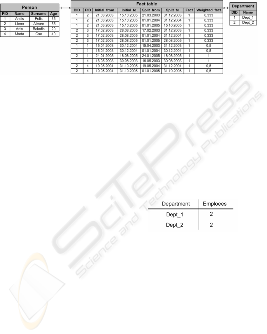
As it is seen from figure 3, the company has two
different departments, and four employees are
working there. With these persons contracts of
employment are concluded. The count of employees
in each department during the time is changing.
The time period, where one value will be taken
from to compute the dynamic of changes, is one year
in our example, so the values are 1
st
of January and
31
st
of December. The Splitted facts are made and
the weighted values and the valid time intervals are
assigned according to section 4.1.
In the figure 3 the company has one contract of
employment with the person2 and person3. These
contracts are valid in some parts of all these three
years. For this reason the initial fact is splitted into
three records and weighted values are 1/3 from the
initial value that was 1 as it is the unity splitting.
Fact records for other persons are splitted also
accordingly to previously described ideas.
From the data that are given in the figure 3, it is
quite easy to get two of the most popular reports.
One of them answers on the following question:
“How many employees do we have in our company
on the specified day, grouped by departments.” In
the code (2) an example query is given. This query
returns the number of employees in the company on
1
st
of July 2004 grouped by departments.
Select name, round(sum(weighted_fact))
from Department d, Fact_table f
where f.department_id=d.department_id
and ‘01.07.2004’ between (initial_from
and initial_to) group by name
(2)
As the weighted fact values are almost not
possible or at least not easy to store in a format 1/3
or 1/7, the weighted fact values normally are finite
decimal numbers. When the weights are
summarized, it is not possible to get whole numbers.
Some additional solutions can be introduced for not
losing some data because of rounding,
– Weighted fact can be stored using big precision.
– The fact can be weighted in not exact values.
This means that instead of three equal values of
0.33 when splitting unity fact, it is possible to
substitute one of the facts from the fact group
with 0.34. In such a way the total for these
weights will be exactly the beginning value
which in this case was one.
– To use views with partly summarized values.
This approach also makes these solutions more
understandable for data warehouse users.
The results of query in the code (2) that are
referencing the data structures from figure 4 are
given in the table 1.
Table 1: Company’s employees’ count in 1
st
of July 2004.
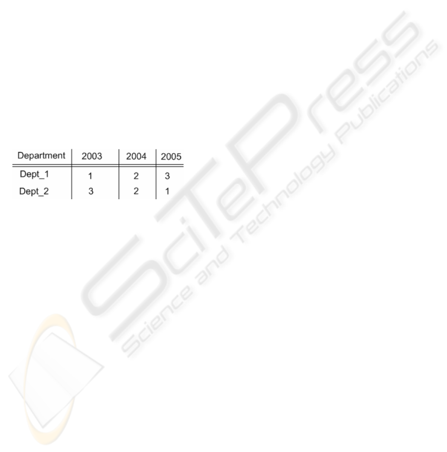
Second typical data warehouse report that is
possible to get using splitted facts is the change
dynamics of the employees count across several
years. This means that we would like to get
employees count for each department in each year’s
specified date. Normally this date is given as a
parameter. In the code (3) a query is shown against
figure’s 3 data structures. This query returns the
distribution of the employees in each year
separately.
Select name, sum(fact),
year(splitted_from) from Department d,
Fact_table f where f.department_id=
d.department_id and ‘01.07’ between
(day_month(splitted_from) and
day_month(splitted_to)) group by name,
year(splitted_from)
(3)
If we are building such queries, it is not possible
to manage without different time functions. First of
Figure 3: Star schema filled with data.
SPLITTING FACTS USING WEIGHTS
257
all the year has to be separated from the full date. On
the other hand in real life situation in the fact table
the foreign keys to the time dimension are stored.
But in the time dimension usually is a column called
“Year”. This is a reason why we can avoid the
function year. In any case it is not the difficult one
as function that extracts year from full date usually
is built in DBMS. The mandatory function in this
query is the one that can extract day and month from
the full date. In this example we are calling it
day_month. In a lot of situations it can be avoided
using substrings, concatenations and data type
translation functions. A little bit similar is the
function between. This function in DBMS level is
defined for built in data types like date, integer, real.
This is why it should be overloaded in a way that
between can work with partial date as the year this
time is not important.
The results from query in code (3) are presented
in table 2.
Table 2: Company’s employees’ count change dynamic
calculated on each year 1
st
of July.
When the fact splitting is used, the record count
in fact table is growing. It is not possible to predict
the percentage of growth for all situations. For each
fact table it can be very different. It depends on the
nature of facts, that is, how slow evolving they are.
The second point is, how long is the period, from
which we want to take the value for making
dynamics. It can be day, hour, month or year. In our
project, where the contracts of employment are
stored, the record count grew about three times.
Other benefit, which can be got by combining two
different facts into one fact table, is less storage
space. This is not only because we do not need to
make almost the same fact tables with almost the
same primary keys. Also the indexes should not be
duplicated.
6 CONCLUSION
We introduced solutions for implementing splitted
facts using weights in this paper. There were also
given an example of how to use such structures in
real world situation. However, fact splitting can be
used in other situations as well. One of them is fact
splitting in bitemporal data warehouses. The facts
can be splitted accordingly to transaction time and
validity time overlapping intervals. In that way we
could analyze data looking at events history from
different perspectives.
Other situation when splitting facts could be
appropriate solution is having inconsistent data from
different data sources that has to be integrated. Such
situations should be researched more closely.
REFERENCES
Abelló, A., Samos, J., and Saltor, F. 2001. Understanding
facts in a multidimensional object-oriented model. In:
Proc. of the 4th ACM international Workshop on Data
Warehousing and OLAP. ACM Press, 32-39.
Abelló, A., Martin C. 2003. A Bitemporal Storage
Structure for a Corporate Data Warehouse. In: Proc.
of the 5th Int. Conf. of Enterprise Information Systems
(ICEIS 2003), 177-183.
Chen, C., Cochinwala, M., and Yueh, E. 1999. Dealing
with slow-evolving fact: a case study on inventory
data warehousing. In: Proc. of the 2nd ACM
international Workshop on Data Warehousing and
OLAP. ACM Press, 22-29.
Eder, J. , Koncilia, C. , and Kogler, H. 2002. Temporal
data warehousing: business cases and solutions. In:
Proc. of the International Conference on Enterprise
Information Systems (ICEIS'02), Spain, 81-88.
Hüsemann, B. , Lechtenbörger, J., and Vossen., G. 2000.
Conceptual Data Warehouse Design. In Proc. of the
International Workshop on Design and Management
of Data Warehouses (DMDW 2000), CEUR-WS
(www.ceur-ws.org).
Inmon, W.H.. 1996. Building the Data Warehouse, John
Wiley.
Jarke, M., Lanzerini, M., and Vassiliou, Y. 2002.
Fundamentals of Data Warehouses, Berlin:Springer.
Kimball, R. 1996. The Data Warehouse Toolkit: Practical
Techniques for building Dimensional Data
Warehouses. Jon Wiley & Sons.
Kimball, R., Reeves, L., Ross, M., and Tthornthwaite, W.,
1998. The Data Warehouse Lifecycle Toolkit: Expert
Methods for Designing, Developing and Deploying
Data Warehouses, New York: Jon Wiley & Sons.
Kimball, R. and Ross M., 2002. The Data Warehouse
Toolkit: The Complete Guide to Dimensional
Modeling, John Wiley.
Song, I.-Y. , Rowen, W. , Medsker, C. , and Ewen,E.
2001. An Analysis of Many-to-Many Relationships
Between Fact and Dimension Tables in Dimensional
Modeling. In Proc. of the Int. Workshop on Design
and Management of Data Warehouses (DMDW'2001).
CEUR-WS (www.ceur-ws.org).
ICEIS 2006 - DATABASES AND INFORMATION SYSTEMS INTEGRATION
258
