
LEARNING NONLINEAR MANIFOLDS OF DYNAMIC TEXTURES
Ishan Awasthi
Department of Electrical and Computer Engineering, Rutgers University, Piscataway, NJ, USA
Ahmed Elgammal
Department of Computer Science, Rutgers University, Piscataway, NJ, USA
Keywords: Texture, Dynamic Texture, Image-based Rendering, Non Linear Manifold Learning.
Abstract: Dynamic textures are sequences of images of moving scenes that show stationarity properties in time. Eg:
waves, flame, fountain, etc. Recent attempts at generating, potentially, infinitely long sequences model the
dynamic texture as a Linear Dynamic System. This assumes a linear correlation in the input sequence. Most
real world sequences however, exhibit nonlinear correlation between frames. In this paper, we propose a
technique of generating dynamic textures using a low dimension model that preserves the non-linear
correlation. We use nonlinear dimensionality reduction to create an embedding of the input sequence. Using
this embedding, a nonlinear mapping is learnt from the embedded space into the image input space. Any
input is represented by a linear combination of nonlinear bases functions centered along the manifold in the
embedded space. A spline is used to move along the input manifold in this embedded space as a similar
manifold is created for the output. The nonlinear mapping learnt on the input is used to map this new
manifold into a sequence in the image space. Output sequences, thus created, contain images never present
in the original sequence and are very realistic.
1 INTRODUCTION
Our aim is to design an algorithmic framework that
allows the creation of photorealistic, yet, arbitrarily
long sequences of images for a dynamic scene,
based on a short input sequence of a similar scene.
Variously referred to as Dynamic Textures (Soatto
et al, 2001), Video Textures (Schödl et al., 2000) or
Temporal Textures (Szummer et al., 1996), these are
image sequences that model motion patterns of
indeterminate spatial and temporal extent. Waves in
water, grass in wind, smoke, flame, fire, waterfall,
etc. are a few examples of phenomena that fall in
this category.
There are two basic ways to approach this problem,
a) Physics based rendering
b) Image based rendering
Physics based rendering is primarily focused on
creating a physical model derived from the standard
principles, to recreate the dynamics of the system.
To make the output a little more realistic,
approximations are then introduced and the model is
simulated to synthesize an output sequence. The
main advantage of this technique is that it provides
extensive manipulation capability and an avenue to
use the model for scientific calculations. But this
technique suffers from the disadvantage of being
computationally expensive and being less
photorealistic. Perry and Picard (Perry et al., 1994)
and Stam et al. (Stam et al., 1995) depicted the
power and use of physics based models to
synthesize sequences of gaseous phenomena like
fire, flame, smoke, etc. Hodgins et al. (Hodgins et al,
1998) proposed a physical model for synthesizing
and studying walking gaits. These provided
sequences which could be easily manipulated but
failed to produce visually appealing outputs.
Image based rendering techniques are focused on
the creation of visually appealing and realistic
output sequences. These could either follow a
procedural technique generating synthetic images by
clever concatenation or repetition of image frames.
Or, these could be based on a model of the visual
signal of the input sequence. Schödl et al. (Schödl
et al., 2000) used a procedural technique to carefully
choose sub-loops of an original video sequence and
243
Awasthi I. and Elgammal A. (2006).
LEARNING NONLINEAR MANIFOLDS OF DYNAMIC TEXTURES.
In Proceedings of the First International Conference on Computer Vision Theory and Applications, pages 243-250
DOI: 10.5220/0001378202430250
Copyright
c
SciTePress

create new sequences. They found frames
representing ‘transition points’, in the original
sequence. By selecting the frames that did not end
up at ‘dead-ends’, that is, places in the sequence
from which there are no graceful exits, they created
very realistic output sequences. But they only
replayed already existing frames, and had to rely on
morphing and blending to compensate for visual
discontinuities. Sequences which did not have
similar frames well spaced temporally, were very
difficult to be synthesized. Many natural processes
like fluids were thus, hard to synthesize. Kwatra et
al. introduced a new seam finding and patch fitting
technique for video sequences. They represented
video sequences by 3D spatio-temporal textures.
Two such 3D textures could be merged by
calculating a 2D surface which could act as the
optimal seam. However like in (Schödl et al., 2000),
they first found transition points by comparing the
frames of the input sequence. Then in a window of a
few frames around this transition they found an
optimal seam to join the two sequences, represented
as 3D textures. Since they rely on transitions, they
sometimes need very long input sequences to find
similar frames and a good seam. Both (Schödl et al.,
2000) and (13), offered little in terms of editability
as the only parameter that could be controlled was
the length of the output sequence. Simple control
like slowing down or speeding up could not be
achieved. It was only techniques based on a model
of the visual signal in the input images, that
provided this opportunity to control various aspects
of the output. Szummer and Picard (Szummer et al.,
1996) suggested a STAR model for generating
temporal textures using an Auto Regressive Process
(ARP). Fitzgibbon (Fitzgibbon et al., 2001)
introduced a model based technique of creating
video textures by projecting the images into a low-
dimensional eigenspace, and modeling them using a
moving average ARP. Here, some of the initial
eigenvector responses (depicting non-periodic
motions, like panning) had to be removed manually.
Soatto et al. (Soatto et al, 2001) produced similar
work. They modeled dynamic textures as a Linear
Dynamic System (LDS) using either a set of
principal components or a wavelet filter bank. They
could model complex visual phenomena such as
smoke and water waves with a relatively low
dimensional representation. The use of a model not
only allowed for greater editing power but the
output sequences also included images that were
never a part of the original sequence. However, the
outputs were blurry compared to those from non-
procedural techniques and for a few sequences the
signal would decay rapidly and the intensity gets
saturated. Yuan et al. (Yuan et al., 2004) extended
this work by introducing feedback control and
modeling the system as a closed loop LDS. The
feedback loop corrected the problem of signal
decay. But the output generated was still blurry.
This is because these models assume a linear
correlation between the various input frames.
In this paper, we propose a new modeling
framework that captures the non-linear
characteristics of the input. This provides clear
output sequences comparable to those of the
procedural techniques while providing better control
on the output through model parameters. The
organization of the paper is as follows: Section 2
describes the mathematical framework that forms
the basis of our model. In section 3, we provide a
brief overview of Non-Linear Dimensionality
Reduction (NLDR). Section 4 describes the
technique used to model the dynamics of the
sequence in the embedded space. In section 5, we
describe the methodology of transforming the model
from the low dimension embedding space to the
observed image space. Finally, section 6 presents the
results of using our framework on a diverse set of
input image sequences.
2 MODEL FRAMEWORK
In this section we summarize the mathematical
framework that we use for modeling the dynamic
texture. The existing image based techniques model
the input visual signal ((Soatto et al,
2001),(Fitzgibbon et al., 2001),(Szummer et al.,
1996)) for creating dynamic textures, using a linear
dynamic system of the following form:
1
,(0,)
,(0,)
tttt v
tttt w
xAx vv
yCxww
−
=
+ Σ
=
+ Σ
∼
∼
Here,
n
t
y
R
∈
is the observation vector;
,
r
t
x
Rr n
∈
<<
is the hidden state vector, Ais the
system matrix;
C is the output matrix and ,
tt
vware
Gaussian white noises driving the system. In such a
system, the observation is a linear function of the
state. The limitation of this system is that this
captures only the linear correlation between
subsequent images. The lack of non-linear
characteristics, lead to an output sequence that is not
as crisp and detailed as the input.
VISAPP 2006 - IMAGE ANALYSIS
244

We, propose a new model based on non-linear
dimensionality reduction, which overcomes this
shortcoming. The state representation is nonlinearly
related to the observation and therefore, the
parameters learnt, effectively model the non-
linearities relating to substructures and small
movements in the input sequence. The framework
we propose is:
1
,(0,)
() , (0, )
tttt v
tttt w
xAx vv
yBx ww
ψ
−
= + Σ
=+ Σ
∼
∼
Where,
n
t
y
R∈ is the observation vector;
,
r
t
x
Rr n∈<<
is the hidden state vector, Ais the
system matrix; B represents the coefficients of non-
linear mappings;
()
x
ψ
is a function incorporating
the basis functions to be used with
B
to define the
non-linear mapping and
,
tt
vware Gaussian white
noises driving the system.
We use NLDR using Locally Linear Embedding
(LLE)(Roweis et al., 2000) and isometric feature
mapping (Isomap) (Tenenbaum et al., 2000), to
achieve a nonlinear embedding of the sequence.
Given such an embedding, we explicitly model the
transitions using a spline curve. This models the
nonlinear manifold of the texture. Using the
embedding, a RBF nonlinear mapping is fitted to the
observation which leads to the nonlinear observation
model in section 5-equation (2).
3 NON-LINEAR EMBEDDING
The model based approaches use dimensionality
reduction to extract compact representations of
relevant characteristics defining the data variability.
Two popular forms of dimensionality reduction are
principal component analysis (PCA) and
multidimensional scaling (MDS). Both PCA and
MDS are eigenvector methods that model variations
in high dimensional data. PCA, finds a low-
dimensional embedding of the
data points that best
preserves their variance
as measured in the high-
dimensional input
space by computing the linear
projections in the directions of greatest variance
using the top eigenvectors of the data covariance
matrix. Metric MDS, computes the low dimensional
embedding that best preserves pair-wise distances
between data points. If these distances correspond to
Euclidean distances, the results of metric MDS are
similar to those of PCA. Both methods are simple to
implement, and their optimizations do not involve
local minima, making these a popular choice despite
their inherent limitations as linear methods.
However, most scenes of simple natural phenomena
depict non-linear dynamics and linear
dimensionality reduction fails to capture the factors
defining these non-linear characteristics. To
overcome this shortcoming, we use non-linear
dimensionality reduction to project the images into a
low dimensionality embedding space. This is
achieved using either the LLE or the Isomap
algorithm. The following sub-sections discuss these
methods in brief.
3.1 Locally Linear Embedding
(LLE)
According to the LLE framework (Roweis et al.,
2000), given the assumption that each data point and
its neighbors lie on a locally linear patch of the
manifold (Roweis et al., 2000), each point (image
frame) y
i
can be reconstructed based on a linear
mapping
ij i
j
wy
∑
that weights its neighbors
contributions using the weights w
ij
. In our case, the
neighborhood of each point is determined by its K
nearest neighbors based on the distance in the input
space. The objective is to find such weights that
minimize the global reconstruction error,
2
( ) | | , where i, j = 1 · · · N
iiji
ii
Ew y wy=−
∑
∑
The weights are constrained such that w
ij
is set to 0
if point y
j
is not within the K nearest neighbors of
point y
i
. This will guarantee that each point is
reconstructed
from its neighbors only. The weights obtained by
minimizing the error in the above equation are
invariant to rotations and re-scalings. To make them
invariant to translation, the weights are also
constrained to sum up to one across each row, i.e.,
the minimization is subject to
1
ij
j
w =
∑
. Such
symmetric properties are essential to discover the
intrinsic geometry of the manifold independent of
any frame of reference. Optimal solution for such
optimization problem can be found by solving a
least-squares problem as was shown in (Roweis et
al., 2000). Since the recovered weights W reflect the
intrinsic geometric structure of the manifold, an
LEARNING NONLINEAR MANIFOLDS OF DYNAMIC TEXTURES
245

embedded manifold in a low dimensional space can
be constructed using the same weights. This can be
achieved by solving, for a set of points
{,1..}
e
i
X
xRi N=∈ = in a low dimension
space, wherein,
ed<< , and that minimize:
2
() | |
iiji
E
xxwx=−
∑∑
where i, j = 1· · ·
N, and, the weights are fixed. Solving such problem
can be achieved by solving an eigenvector problem
as was shown in (Roweis et al., 2000).
3.2 Isomap Embedding
Isometric feature mapping (Tenenbaum et al., 2000),
or Isomap, algorithm preserves the pair-wise
distances between points in the image space. It adds
the additional constraint of preserving the intrinsic
geometry of the data as described by the geodesic
manifold distances between all pairs of data points.
For neighboring points, Euclidian distance provides
a good approximation to geodesic distance. For
faraway points, geodesic distance is approximated
by adding up a sequence of “short hops” between
neighboring points. These hops are computed by
finding shortest paths in a graph with edges
connecting neighboring data points. The algorithm
as defined in (Tenenbaum et al., 2000) has three
main steps:
The first step determines which points are neighbors
on the manifold M, based on the distances
(, )
x
dij
between pairs of points i, j in the high dimension,
input space X. It either connects each point to all
points within some fixed radius
e , or to all of its
K
nearest neighbors. These neighborhood relations are
represented as a weighted graph
G over the data
points, with edges of weight
(, )
x
dij between
neighboring points. In its second step, Isomap
estimates the geodesic distances
(, )
M
dij between
all pairs of points on the manifold M by computing
their shortest path distances
(, )
G
dijin the
graph
G
. In the third and final step, MDS is applied
to the matrix of graph distances
{(,)}
GG
Ddij= ,
constructing an embedding of the data in a d-
dimensional Euclidean space
Y
that best preserves
this estimated intrinsic geometry. The coordinate
vectors
i
y
for points inY are chosen to minimize the
cost function:
2
G
E=|| (D ) ( ) ||
Y
L
D
τ
τ
−
Where,
Y
D denotes the matrix of Euclidean
distances
{(,)|| ||}
Yij
dij y y
=
− and
2
|| ||
L
A the
2
L matrix norm =
2
,
ij
ij
A
∑
. The
τ
operator
converts distances to inner products, which uniquely
characterize the geometry of the data in a form that
supports efficient optimization. The global minimum
of Eq. 1.2 is achieved by setting the coordinates
i
y
to the top d eigenvectors of the matrix ()
G
D
τ
.
4 LEARNING DYNAMICS
Non-Linear dimensionality reduction provides us a
low dimensional embedding that closely captures the
dynamics of the input sequence. Each input frame
resides as a node on the embedded manifold. A new
sequence, with similar dynamics, will also have a
similar low dimensional embedding. The first step
towards the creation of the output sequence is the
creation of the output manifold in the same
embedding space. To do so, first a model of the
embedding is created and then this model is used to
create a new manifold.
4.1 Modeling the Embedded
Manifold
The non-linear dimensionality reduction techniques
are used to create an embedding of the input
sequence in 3D space. The embedded manifold is
then modeled as a 3d-spline. This is done by
assuming consecutive frames to be equidistant in
time and, using the 3D coordinates of each frame
within the embedding space, to construct a piece-
wise polynomial in each dimension. Thus, at any
time
t a point (, ,)
ttt
Ax y z on the embedding can
be represented by
() ( (), (), ())
f
t PPx t PPy t PPz t
=
Where,
PPx, PPy and PPz are the piecewise
polynomials fitting the x, y and z co-ordinates of the
frames of the input sequence in the embedding
space.
4.2 Creating the Output Manifold
The embedding manifold for the output is created by
using the manifold for the input as a guide and
VISAPP 2006 - IMAGE ANALYSIS
246
walking through the embedding space. If T is the
time used for an input sequence with
m input
frames, the average time-step between consecutive
frames is
/
av
TTm
=
Starting at the first frame, and moving along the
spline at steps equal to
av
T would result in an exact
trace of the input sequence. In order, to create a
unique sequence, some noise is added to the time
step between two consecutive frames. Also to allow
for a rate of change of speed, an acceleration factor
α
is also introduced. Thus, the time step for the
embedding for the output sequence can be
represented as
step av
TT
α
γ
=+
The use of
s
tep
T ensures the unique positioning of
nodes representing frames of the output sequence,
along the embedding manifold. However, the actual
trajectory of the manifold for the output sequence
still remains the same as that of the input sequence.
In order to add variability to the trajectory for the
output sequence, gaussian noise is also added to the
3d co-ordinates calculated by the piecewise
polynomials
PPx, PPy and PPz . The new
spline function now becomes:
((),(),())
new n x n y n z
f f PPx T PPy T PPz T
μ
μμ
=+ + +
Where,
x
μ
,
y
μ
and
z
μ
represent Gaussian noise
along
x
,
y
and z co-ordinates respectively. Thus,
from a position at time
cur
T on the output manifold,
the next position is calculated as:
()
cur cur step
new new cur
TTT
Pos f T
=+
=
(1)
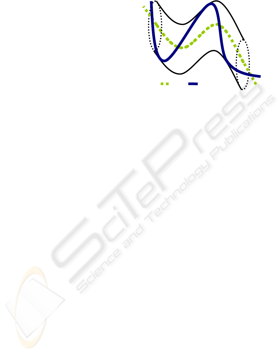
Using, (1) we are able to create a new manifold
within the 3d-embedding space that is restricted to
within a cylindrical, twisted, shell with the manifold
of the input sequence forming the axis of this shell.
Figure 1.
5 OBSERVATION MODEL
Once the manifold in the embedding space has been
modeled, we need to map points from the low
dimensional embedding space into the high
dimensional visual input space. In order to learn
such nonlinear mapping, a Radial basis function
interpolation framework is used. In the Radial basis
functions interpolation framework, the manifold is
represented in the embedding space implicitly by
selecting a set of representative points along the
manifold.
Let the set of representative input instances be
d
i
Y = {y R i = 1, · · · ,N}∈ and let their
corresponding points in the embedding space be
e
i
X = {x R , i = 1, · · · ,N}∈ where e is the
dimensionality of the embedding space (e.g. e = 3 in
our case). We can solve for multiple
interpolants
:
ke
f
RR→ , where k is k -th
dimension (pixel) in the input space and
k
f
is a
radial basis function interpolant, i.e., we learn
nonlinear mappings from the embedding space to
each individual pixel in the input space. The
functions used are generally of the form:
k
f() () (| |)
N
kk
ii
i
x
px w xx
φ
=+ −
∑
where
(.)
φ
is a real valued basis function,
i
w are
real coefficients,
|.|is the norm on
e
R
(the
embedding space) and
k
p
is a linear polynomial
with coefficients
k
c
. The basis function we have
Output
Manifold
Input
Manifold
LEARNING NONLINEAR MANIFOLDS OF DYNAMIC TEXTURES
247

used is the thin-plate spline
2
( ) log( )uu u
φ
= . The
whole mapping can be written in a matrix form as
() . ()
f
xBx
ψ
= (2)
Where
B
is a (1)dNe×++dimensional matrix
with the
k -th row
1
[ ... ]
T
kkk
N
wwc and the vector
()
x
ψ
is
TT
1N
[ (|x - x |) · · · (|x - x |) 1 x ]
φφ
The matrix
B
represents the coefficients for
d different nonlinear mappings, each from a low-
dimension embedding space into real numbers. To
insure orthogonality and to make the problem well
posed, the following additional constraints are
imposed
1
( ) 0, 1,...,
N
ij
i
wp x j m
=
==
∑
where
j
p
are the linear basis of
p
. Therefore the
solution for
B
can be obtained by directly solving
the linear systems
(1)
0
0
T
T
ed
Y
AP
B
P
+×
⎛⎞
⎛⎞
=
⎜⎟
⎜⎟
⎝⎠
⎝⎠
Where,
(| |), , 1...
ij j i
AxxijN
φ
= − = , P is a
matrix with
i
-th row
[1 ]
T
i
x
and Y is
()Nd× matrix containing the input images
1
[ ... ]
T
N
y
y .
6 EXPERIMENTAL RESULTS
The algorithm was tested on various different input
image sequences of varying length. The outputs
were sequences with lengths, four times or greater
than the input. Figure 2 shows the results for four
sequences, each depicting different dynamics. The
output sequences can be viewed online at
http://www.cs.rutgers.edu/~elgammal/DynamicText
ure. The input sequence for each was 70 frames in
length. As can be seen, the synthesized images
maintain both the dynamics and structure of the
input. Depending on the shape of the input manifold,
different approaches are used in generating the
output manifold. The manifolds fell into one of
three broad categories.
6.1 Closed Loop Embedding
Manifold
When, the starting and the ending frames of the
input sequence were either similar or at a small
distance in the 3d-embedding space of the input
manifold, the spline could be modified into a closed
loop. This was achieved by introducing an edge
between the first and the last points on the manifold
(representing the first and the last frame) during the
creation of the output manifold. The Flame, the
Sparkling-ball and the Fountain sequences (Figure 2
(b),(c),(d)) show how the long output sequences,
thus created. The output manifold for these
sequences were created by looping around the
closed loop of the input manifold as many times as
was needed. Figure 3 (b), (c) & (d) show the
manifold for the three sequences respectively.
6.2 Open Ended Embedding
Manifold
When the starting and ending frames were far apart
compared to the average distance between any 2
consecutive frames along the embedded manifold,
closing the loop constituted a big jump and resulted
in a jerk being introduced in the subsequently
synthesized sequence. In such cases, the output
manifold could be created by oscillating between the
two extremes of the spline. However, this solution
could be applied only to image sequences which
already had some oscillation, like the beach and the
turning face sequences. Figure 3 (a),(e) show the
manifold for these, respectively.
6.3 Jerky Embedding Manifold
When, the input sequence comprises of relatively
random and fast motion like in the boiling water
sequence. The image frames are scattered within a
small volume of the embedding space and the spline
model constitutes a lot of sporadic jumps. In such a
sequence, looping back to the first frame after the
last has been reached, allows for a loop to be created
with the associated jerk in the visual image space
blending in with the rest of the jerks that the input
sequence already depicts. Light and High-boiling
water and the wavy river sequence have such a
manifold. The manifold for the boiling water
sequence is shown in Figure 3(f).
VISAPP 2006 - IMAGE ANALYSIS
248
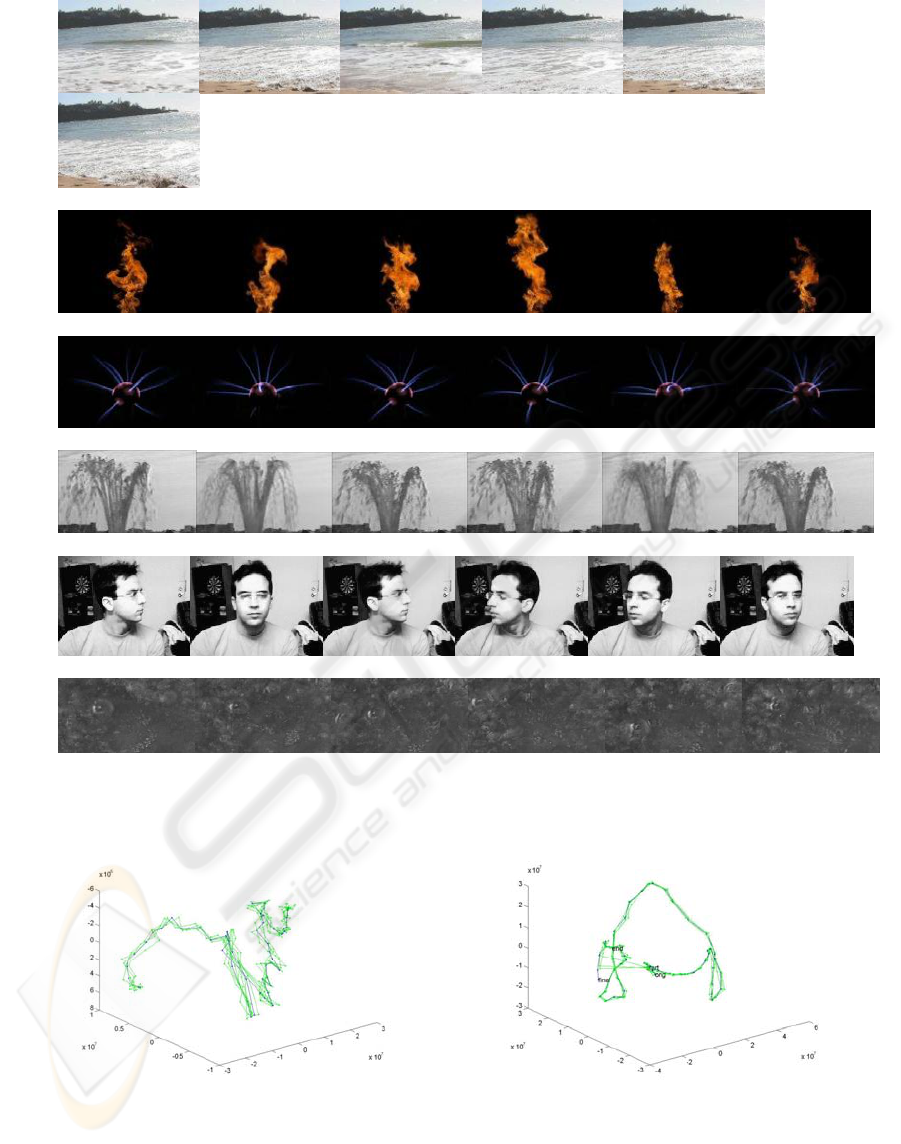
a)
b)
c)
d)
e)
f)
Figure 2: a)Beach, b)Flame, c)Sparkling Ball, d)Fountain, e)Face, f)Boiling Water.
a)Beach
b)Flame
LEARNING NONLINEAR MANIFOLDS OF DYNAMIC TEXTURES
249
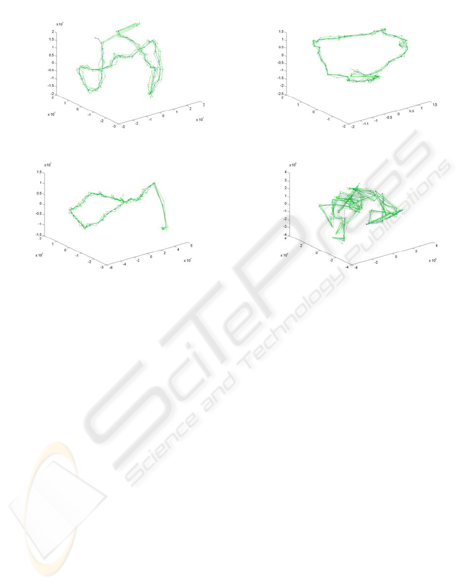
c)Sparkle d)Fountain
e)Face
f)Boilingwater
Figure 3.
REFERENCES
J. Stam and E. Fiume. Depicting fire and other gaseous
phenomena using diffusion processes. In Proc.
SIGGRAPH ’95, pages 129–136, August 1995.
J. K. Hodgins and W. L.Wooten. Animating human
athletes. In Robotics Research: The Eighth
International Symposium, pages 356–367, 1998.
J. Popovićć, S. M. Seitz, M. Erdmann, Z. Popovi´c, and A.
Witkin. Interactive manipulation of rigid body
simulations. In Proc. of SIGGRAPH ’00, pages 209–
218, July 2000.
C. H. Perry and R. W. Picard, ”Synthesizing Flames and
Their Spreading,” Proc. of the 5th Eurographics
Workshop on Animation and Simulation, Oslo,
Norway, Sept. 1994.
A. Schödl, R. Szeliski, D.H. Salesin, I. Essa, Video
textures, in: K.Akeley (Ed.), Siggraph 2000, Computer
Graphics Proceedings, ACMPress/ACM
SIGGRAPH/Addison Wesley/Longman, 2000, pp.
489–498.
A.W. Fitzgibbon, Stochastic rigidity: image registration
for nowherestatic scenes, Proceedings of the Eighth
International Conference On Computer Vision, 2001,
pp. 662–669.
S. Soatto, G. Doretto, Y.N. Wu, Dynamic textures,
International Conference on Computer Vision, 2001,
pp. 439–446.
V. Kwatra, A. Sch¨odl, I. Essa, G. Turk and A. Bobick.
Graphcut Textures: Image and Video Synthesis Using
Graph Cuts. In Proceedings of Siggraph’03, pp. 277-
286, 2003.
M. Szummer and R. W. Picard. Temporal Texture
Modeling. IEEE International Conference on Image
Processing, vol. 3, pp. 823-826, 1996.
L. Yuan, F. Wen, C. Liu, and H.Y. shum, “Synthesizing
Dynamic Texture with Closed-Loop Linear
Dynamical System”, ECCV 2004, LCNS 3022,
pp.603—616, 2004.
S. Roweis and L. Saul, Nonlinear dimensionality
reduction by locally linear embedding, Science 290
(2000), 2323{2326.
J. B. Tenenbaum, V. de Silva, and J. C. Langford, A
global geometric framework for nonlinear
dimensionality reduction, Science 290 (2000),
2319{2323.
VISAPP 2006 - IMAGE ANALYSIS
250
