ADAPTIVE STACK FILTERS IN SPECKLED IMAGERY

Mar

ıa E. Buemi, Marta E. Mejail, Julio C. Jacobo, Mar

ıa J. Gambini

Departamento de Computaci

on. Facultad de Ciencias Exactas y Naturales. Universidad de Buenos Aires

Pabell

on I. Ciudad Universitaria.1428 Buenos Aires. Rep

ublica Argentina

Keywords:

Stack ﬁlter, sinthetic aperture radar, speckle, classiﬁcation.

Abstract:

Stack ﬁlters are a special case of non-linear ﬁlters. They have a good performance for ﬁltering images with

different types of noise while preserving edges and details. A stack ﬁlter decomposes an input image into

several binary images according to a set of thresholds. Each binary image is ﬁltered by using a boolean

function. Adaptive stack ﬁlters are optimized ﬁlters that compute a boolean function by using a corrupted

image and ideal image without noise. In this work the behaviour of an adaptive stack ﬁlter is evaluated for the

classiﬁcation of synthetic apreture radar (SAR) images, which are affected by speckle noise. With this aim

it is carried out a Monte Carlo experiment in which simulated images are generated and then ﬁltered with a

stack ﬁlter trained with one of them. The results of their maximum likelihood classiﬁcation are evaluated and

then are compared with the results of classifying the images without previous ﬁltering.

1 INTRODUCTION

Stack ﬁlters are a special case of non-linear ﬁlters.

They have a good performance for ﬁltering images

with different types of noise while preserving edges

and details. These ﬁlters consist of a decomposition

by thresholds of an input signal obtaining a binary sig-

nal for each threshold. Each binary signal is ﬁltered

using a sliding window. Stack ﬁlters can be gener-

ated using an adaptive algorithm, in such a way that

the so-called stacking property holds. The stack ﬁlter

design method used in this work is based on an algo-

rithm proposed by Yoo et al. (Yoo et al., 1999). In

this paper we study the application of this type of ﬁl-

ter to Synthetic Aperture Radar (SAR) images. SAR

images (Goodman, 1976) and (Oliver and Quegan,

1998) are generated by a coherent illumination sys-

tem and are affected by the coherent interference of

the signal backscatter by the elements on the terrain.

This interference causes ﬂuctuations of the detected

intensity which varies from pixel to pixel. This ef-

fect is called speckle noise. Speckle noise, unlike

noise in optical images, is neither Gaussian nor ad-

ditive; it follows other distributions and is multiplica-

tive. Due to all of this it is not possible to treat these

images using the classical techniques appropiate for

optical image processing. The analysis of this type

of images has been treated in the literature using sev-

eral statistical methods, see for example (Frery et al.,

1999), (Mejail et al., 2001), (Mejail et al., 2003)

and (Mejail, 1999). Under the multiplicative model,

the returned image Z can be thought as two indepen-

dent random variables: the random variable X that

represents the backscatter and the random variable Y

that represent the speckle noise. Different statistical

distributions have been proposed in the literature. In

this work we use the Gamma distribution, Γ, for the

speckle, the reciprocal of Gamma distribution, Γ

−1

for the backscatter, which results in the G

(Frery

et al., 1996) distribution for the return. These distrib-

utions depend on three parameters: α that is a rough-

ness parameter, γ a scale parameter, and n the equiv-

alent number of looks. In this work, we classify an

image into different regions according to their homo-

geneity degree, which will be refered to section 5. Af-

ter ﬁltering, the image data have undergone changes

in their statistical distribution functions. A study of

the kurtosis and the skewness coefﬁcients obtained af-

ter ﬁltering show that the image data follows a more

gaussian distribution. Then, we classify the image by

using the maximum likelihood method and consider

the normal distribution with different parameters for

each region. The structure of this paper is as follows:

section 2 gives an introduction to stack ﬁlters, sec-

E. Buemi M., E. Mejail M., C. Jacobo J. and J. Gambini M. (2006).

ADAPTIVE STACK FILTERS IN SPECKLED IMAGERY.

In Proceedings of the First International Conference on Computer Vision Theory and Applications, pages 33-40

DOI: 10.5220/0001376400330040

 SciTePress

tion 3 describes the ﬁlter design method used in this

work. In section 4 we summarises the G

distribution

for SAR images. In section 5 we exhibit the modiﬁ-

cation undergone by data after applying the ﬁlter, and

also report on the results of the classiﬁcation. Finally,

we present the conclusions in section 6.

2 STACK FILTERS: DEFINITIONS

AND DESIGNING

This section is dedicated to a brief synthesis of stack

ﬁlter deﬁnitions and design. For more details on this

subject, see (Lin and Kim, 1994), (Wendt et al., 1986),

(Astola and Kuosmanen, 1997), (Yoo et al., 1999),

(Coyle and Lin, 1988), (Coyle et al., 1989), (J.Lin

et al., 1990). In the ﬁrst place the necessary deﬁni-

tions are presented to explain this type of ﬁlters.

Deﬁnition 1

The threshold operator is given by T

{0, 1,...,M}→{0, 1}

(x)=



1 si x ≥ m

0 si x<m

, (1)

= T

(x). (2)

According to this deﬁnition, the value of a non-

negative integer number x ∈{0, 1,...,M} can be re-

constructed making the summation of its thresholded

values between 0 and M. The formula corresponding

to this operation is

x =



m=1

. (3)

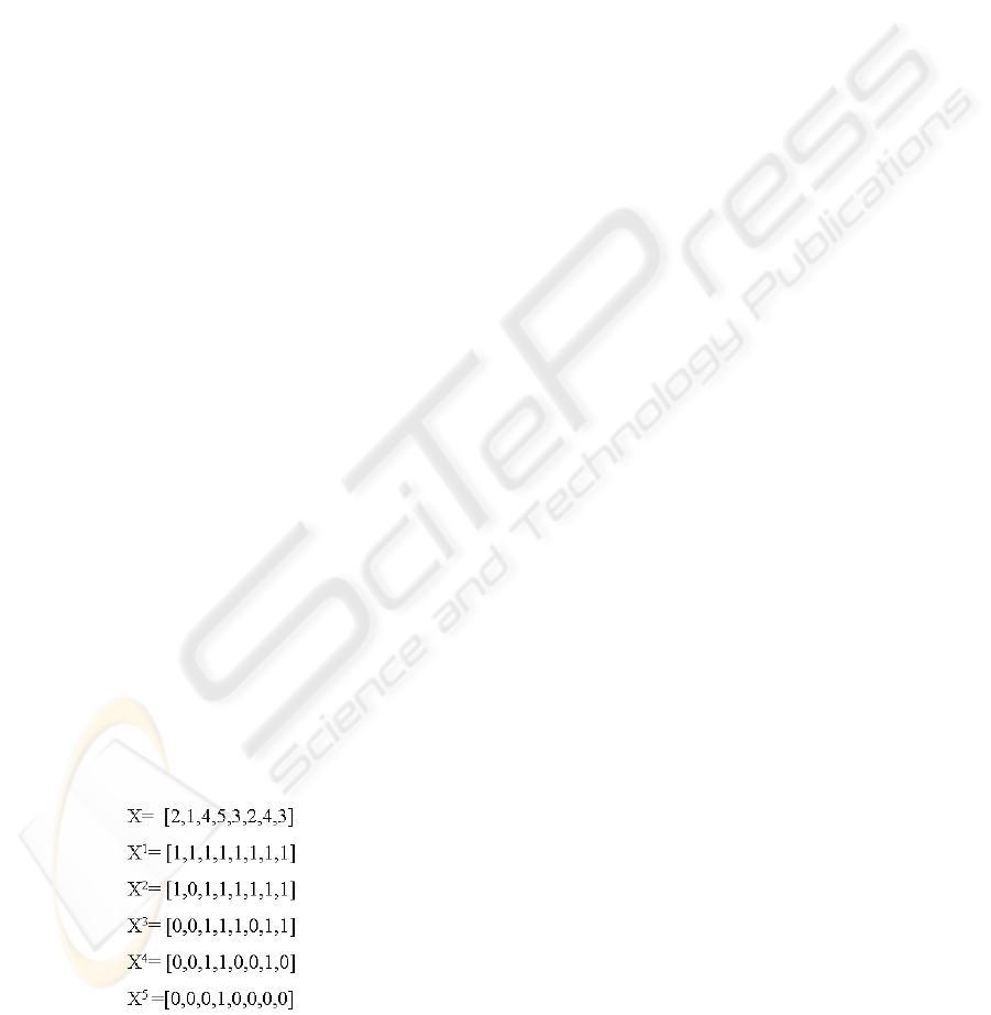
Figure 1 shows a diagram of the threshold decom-

position of a unidimensional signal. The threshold

operator can be extended to bi-dimensional signals.

Figure 1: Example of threshold decomposition.

Deﬁnition 2

Let X=(x

,...,x

n−1

) and Y =(y

,...,y

n−1

)

be binary vectors of length n, then let us deﬁne a re-

lation ≤ given by

X ≤ Y if and only if ∀i, x

≤ y

. (4)

This relation is reﬂexive, anti-symmetric and transi-

tive, generating therefore a partial ordering on the set

of binary vectors of ﬁxed length.

Deﬁnition 3

A boolean function f : {0, 1}

→{0, 1} , where

n is the length of the input vectors, has the stacking

property if and only if

∀X, Y ∈{0, 1}

,X≤ Y ⇒ f (X) ≤ f (Y ) . (5)

Deﬁnition 4

We say that f is a positive boolean function if and

only if it can be written by means of an expression

that contains only non-complemented input variables.

That is,

f (x

,...,x



i=1



j∈P

, (6)

where n is the number of arguments of the function,

K is the number of terms of the expression and the

are subsets of the interval {1,...,N} .



and



are Boolean operators AND and OR. It is possible

to proof that this type of functions has the stacking

property.

If the function f used to ﬁlter an image X fulﬁlls

the stacking property, then from (4) and (5) it is de-

duced that, for two binary images X

and X

, ob-

tained from X as the result of the application of the

thresholds T

and T

respectively, the following im-

plication is valid

i ≥ j ⇒ X

≤ X

⇒ f





≤ f





(7)

A stack ﬁlter is deﬁned by the function S

{0,...,M}

→{0,...,M}, corresponding to

the Positive Boolean function f (x

,...,x

) ex-

pressed in the given form by (6). The function S

can

be expressed by means of

(X)=



m=1

f (T

(X)) (8)

In Figure 2 it can be observed a scheme of aplication

of the ﬁlter to an unidimensional signal. S

represents

the boolean function which ﬁlters each binary thresh-

olded signal and whose outputs are added together to

ﬁnally obtain the ﬁltered signal.

VISAPP 2006 - IMAGE FORMATION AND PROCESSING

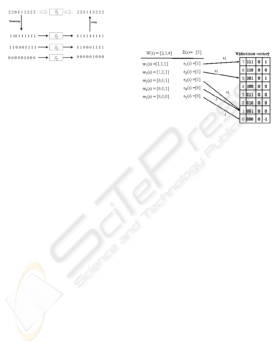
Figure 2: Scheme of the stack ﬁlter applied to an unidimen-

sional signal. S

represents the boolean function applied to

each level.

3 ADAPTIVE ALGORITHMS FOR

STACK FILTERS DESIGN

In this work we applied the stack ﬁlter generated with

the fast algorithm described in (Yoo et al., 1999).

This algorithm, arises as a result of studies on the

methods proposed in (Lin and Kim, 1994) and (J.Lin

et al., 1990). To construct a stack ﬁlter following

any of these methods, a training process that gen-

erates a positive boolean function that preserves the

stacking property, represented by the so-called deci-

sion vector, is carried out. In what follows, the gen-

eration and behaviour of the decision vector is ex-

plained. An image is deﬁned as the set given by:

{(s, v):s ∈ S ⊆ Z

,v ∈ [0,...,M],M ∈ Z},

where s is position and v is the value of a pixel. Let

E and R be two images, where R is the noisy version

of E.AW (s) window is a subimage of R of size

b=r x r centered at position s. Let us deﬁne V as a

dimension vector, and call it the decision vector. In

the training phase of the ﬁlter design, for each s ∈ S,

the data in W (s) are decomposed in M thresholds

obtaining M windows w

(s), i =1,...,M, where

(s) is the ith thresholded version of W (s). Then,

for each s ∈ S in the image E ,a threshold e

(s) is

deﬁned (notice that here e

(s) has dimension 1). If

(s)=1, then the position on V given by w

(s),

considered as a binary number, is increased by one, if

(s)= 0, then the same position is decremented by 1.

Periodically, V is checked to see wether the stacking

property holds. If not, the decision vector V is suit-

able modiﬁed. Finally, the decision vector is trans-

formed into a binary vector that is an implementation

of the positive boolean function f sought. In Figure 3

a ﬁlter training example for a 1D signal, is shown .

Let W (s) be a window of length 3 on the noisy sig-

nal, centered at position s, and let E(s) be the value of

the noiseless signal at the same position. In this case,

W (s)=[2, 1, 4], E(s) = [3] and thresholds varying

between 1 and 5 are considered. The decision vector

V is of size 2

=8and is represented by the table that

contains at the ﬁrst column indices expressed in deci-

mal notation, at the second column indices expressed

in binary notation, at the third column the vector val-

ues after n iterations and at the fourth column the vec-

tor values after the n +1iteration.

Figure 3: Scheme of the generation of the stack ﬁlter.

The training of this stack ﬁlter consists of the al-

ternate application of two different stages: a stage in

which the decision vector is modiﬁed according to the

scheme indicated in Figure 3, and a stage in which the

stacking property is checked and enforced on the de-

cision vector.

4 SAR IMAGES. THE

MULTIPLICATIVE MODEL

In this section we introduce the statistical laws com-

monly used under the multiplicative model for Syn-

thetic Aperture Radar (SAR) images. The multiplica-

tive model considers the image returned by the SAR,

named Z, as a product of two independent random

variables, one corresponding to the backscattter X

and the other one corresponding to the speckle noise

Y,so

Z = XY. (9)

Where we suppose independence among the random

variables corresponding to each image pixel. We can

write formula (9) for each pixel (i, j) of an image of

size M × N as:

i,j

= X

i,j

, 0 ≤ i ≤ M − 1, 0 ≤ j ≤ N − 1.

(10)

The format of the SAR image (complex, amplitude or

intensity) determines the distribution followed by the

speckle noise random variables Y

i,j

. These variables

are i.i.d and the equivalent number of looks n is their

only statistical parameter. On the other hand, the type

of target each pixel belongs to (forest, pasture, crops,

ADAPTIVE STACK FILTERS IN SPECKLED IMAGERY

city) determines de most appropiate distribution for

each of the backscatter random variables X

i,j

4.1 Speckle Distribution

The speckle noise comes from the coherent addition

of individual returns produced by elements present in

each resolution cell. So, for example, in an image

corresponding to a scene of land covered by vegeta-

tion, the returns from the elements of the plants and

the ground are added taking into account the phase,

yielding as a result a complex number. In an ampli-

tude SAR image, the gray level of each pixel is the

module of the this complex number. In an intensity

SAR image, the gray level of each pixel is the square

of this magnitude.

For every pixel, the model for the speckle noise is

the Γ(n, 2n) distribution, where n is the equivalent

number of looks. Then, within this model the density

function for the speckle noise Y is given by

(y)=

Γ(n)

n−1

−ny

,y≥ 0. (11)

In SAR images the minimun value for n is 1. This

value corresponds to images generated without mak-

ing the average of several looks. Images generated in

this manner are noiser than those generated with more

number of looks, but they have better azimuth resolu-

tion and, therefore, potencially more information. We

can suppose that the parameter n is known or that it

can be estimated at an initial stage of the image analy-

sis. Therefore, although in theory it would have to be

an integer number, in practice it is necessary to con-

sider it as a real number for the case in which it is

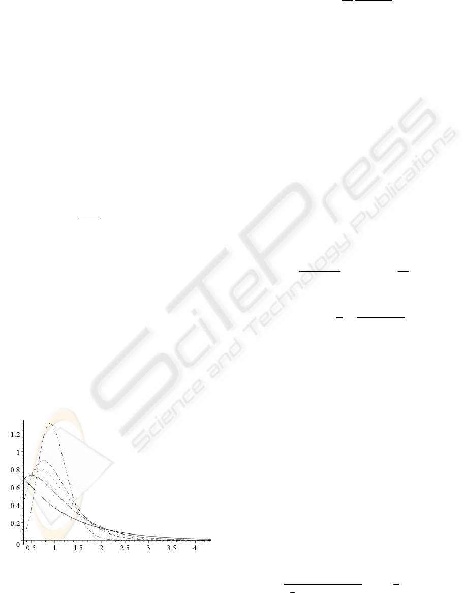
estimated from the data. Figure 4 shows the curves

corresponding to the speckle distribution for different

values of n. The moments of the speckle distribution

Figure 4: Curves of the Γ distribution corresponding to

speckle for number of looks equal to: 1 (solid), 2 (dashes),

3(dots), 4 (dot-dash) and 10 (dot-dot-dash).

are given by:

E[Y

Γ(n + r)

Γ(n)

(12)

where r is the moment order and n ≥ 1 is the number

of looks.

4.2 Backscatter Distribution

There are several models for the backscatter, that is,

different statistical distributions exist for the random

variables X

i,j

. From the results presented in (Frery

et al., 1996) it is possible to consider the Generalised

Inverse Gaussian distribution as a general model for

the backscatter. This distribution is very general and

allows us to describe many different targets, but from

an analitical and numerical point of view the estima-

tion of its parameters is very complex and unstable.

This distribution has various particular cases, one of

which: the Inverse Gamma distribution, is of special

interest to this work. This distribution is proposed as

a universal model for SAR data and it leads to the G

distribution for the return. The Inverse Gamma dis-

tribution, called Γ

−1

, is characterised by the density

function given by

(x)=

Γ(−α)

α−1

exp



−



, (13)

and its moments are expressed as

E [X





Γ(−α − r)

Γ(−α)

, (14)

where α<0 and |α| >r. In Figure 5 we can see the

curves corresponding to a Γ

−1

density function as we

vary the α parameter keeping the mean value equal to

one.

4.3 Distributions for the Return

The distribution corresponding to the return Z,is

ﬁxed by the distribution of the backscatter X and

the distribution of the speckle Y . Given that Z =

XY and that these random variables are independent,

(z) can be calculated as

(z)=



Z|Y =y

(z) f

(y) dy, (15)

where f

Z|Y =y

is the density for the return Z con-

sidering X = x constant and f

the density func-

tion of the speckle Y . For the random variable corre-

sponding to the return (intensity format) we have that

Z ∼G

(α, γ, n), and the density function is given by

(z)=

Γ(n − α)





Γ(−α)Γ(n)

n−1



+ nz



α−n

(16)

VISAPP 2006 - IMAGE FORMATION AND PROCESSING

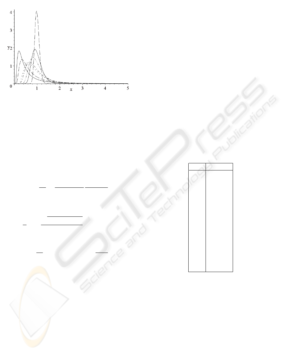
Figure 5: Curves of Γ

−1

distribution with mean value

equal to one and α equal to: −1.5 (solid), −2 (dash), −4

(dots), −5 (dot-dash), −10 (dot-dot-dash), −20 (solid) y

−100(dash).

with α<0, γ>0 and n ≥ 1. Given the indepen-

dence between the backscatter X and the speckle Y ,

the moments of the return Z are the product of the

moments of X and the moments of Y (equations (14)

and ( 12)) yielding

E [Z





Γ(−α − r)

Γ(−α)

Γ(n + r)

Γ(n)

, (17)

recalling that this moments are ﬁnite for −α>r. The

variation coeﬁcient is given by

= −



α (α + n +1)

, α<− (n +1),

where

α (α + n +1), µ =

−αγ

This distribution was proposed in (Frery et al., 1996)

as a model for extremely heterogeneous data, but its

utility for description of a great variety of natural and

artiﬁcial targets was veriﬁed, which resulted in its be-

ing proposed as a universal model for SAR data.

5 RESULTS

This section is dedicated to show the results of apply-

ing a stack ﬁlter to synthetic SAR images. These im-

ages are generated in such a way that their data have

different degrees of homogeneity. We consider differ-

ent values of the α parameter and we compute the γ

parameter so that the mean value of the data is unitary.

The α parameter corresponds to image roughness (or

heterogenity). It adopts negative values, varying from

−∞ to 0.Ifα is near 0, then the image data are

extremely heterogeneous (for example: urban areas),

and if α is far of the origin then the data correspond

to a homogeneous region (for example: pasture ar-

eas), the values for forests and crops lay in-between.

The parameter γ is a scale parameter. Finally, in order

to evalute the behaviour of the ﬁters we carried out

a maximun likelihood classiﬁcation. The results are

analysed in the classiﬁed images, within this images

we compare the ﬁltered and the non-ﬁltered images.

5.1 Statistical Analysis

An important task in statistical analysis is the char-

acterization of the mean value and the variability of

a data set. To this end, the behaviour of some sta-

tistics for ﬁltered and non-ﬁltered images, are com-

pared. Fifteen 100 × 100 images of G

distributed

data were generated using the values of α and γ given

in Table 1. In order to design the stack ﬁlter, an im-

age formed with the mean values of each region, as

described in section 3, was used.

Table 1: Values of α and γ used in the experiment.

α γ

-1.5 1.00000

-2.0 1.62114

-2.5 2.25000

-3.0 2.88202

-3.5 3.51562

-4.0 4.15012

-4.5 4.78516

-5.0 5.42056

-5.5 6.05621

-6.0 6.69205

-6.5 7.32802

-7.0 7.96409

-7.5 8.60024

-8.0 9.23646

-8.5 9.87273

Examples of these images are shown in Figure 6.

This ﬁgure shows the results of applying a 5 × 5 win-

dow size ﬁlter to a group of images. Figures 6(a), 6(c)

and 6(e) correspond to the original speckled images

and ﬁgures 6(b), 6(d) and 6(f) correspond to the ﬁl-

tered images.

A statistical tool for characterizing the signal to

noise ratio is the variation coefﬁcient, deﬁned as

the quotient between the standard deviation and the

mean value: C

=σ/µ. The values of this coefﬁcient

for ﬁltered and non-ﬁltered images are given in Ta-

ble 2. The values corresponding to the ﬁltered images

are lower than the values corresponding to the non-

ﬁltered images, indicating that the effect of ﬁltering

was a decrease in the speckle noise. It can also be

seen that the value of the variation coefﬁcient C

ADAPTIVE STACK FILTERS IN SPECKLED IMAGERY

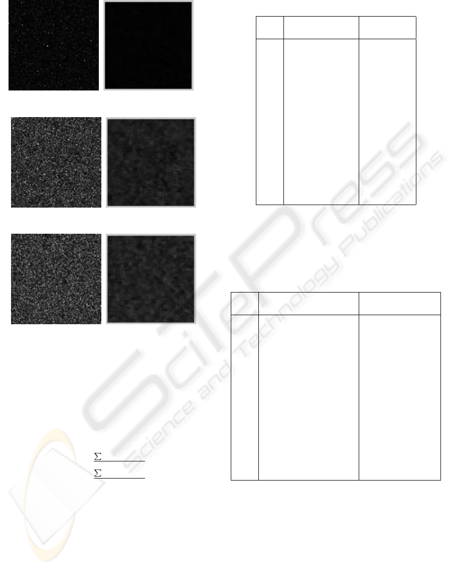
(a) α=−1.5 (b) Filtered image

(e) α=−8.5 (f) Filtered image

Figure 6: Synthetic images (left) and their corresponding

ﬁltered images (right).

lower when the α parameter is lower for both, ﬁltered

and non-ﬁltered images. In order to assess the nor-

mality of the data, the skewness and kurtosis statistics

were used. They are deﬁned by

SK =

i=1

−

Y )

(N−1)s

K =

i=1

−

Y )

(N−1)s

where, Y

,...,Y

are univariate data,

Y is the

mean value, s is the standard deviation, and N is the

sample size. For a normal distribution, the skewness

SK is zero (symmetric density) and the kurtosis K is

The distribution of the data is modiﬁed when they

are ﬁltered. If we consider the skewness and the kur-

tosis as a measure of asymmetry and peakedness be-

tween the data and the density, we can state that the

data are more Gaussian after ﬁltering. This can be

seen in Tables 3 and 4 where the skewness and the

kurtosis for each α value are shown.

Table 2: Variation coefﬁcients.

α C

non-ﬁltered C

ﬁltered

images images

-1.5 1.020400 0.327207

-2.0 0.803039 0.251616

-2.5 0.738860 0.256685

-3.0 0.685162 0.240635

-3.5 0.668856 0.239666

-4.0 0.637395 0.230422

-4.5 0.612268 0.223510

-5.0 0.613924 0.227741

-5.5 0.598406 0.224422

-6.0 0.591566 0.221399

-6.5 0.588123 0.217759

-7.0 0.571000 0.215808

-7.5 0.585607 0.216695

-8.0 0.577546 0.221254

-8.5 0.577740 0.216642

It can be noticed that, the more heterogeneous the

non-ﬁltered data are, that is α closer to 0, the higher

the values for the skewness and kurtosis.

Table 3: Skewness.

α Skewness non-ﬁltered Skewness ﬁltered

images images

-1.5 5.79204 0.542360

-2.0 2.71243 0.452572

-2.5 2.17279 0.354620

-3.0 2.06542 0.404203

-3.5 1.79158 0.396256

-4.0 1.56213 0.287269

-4.5 1.30829 0.283221

-5.0 1.18022 0.339163

-5.5 1.15137 0.323194

-6.0 1.15225 0.261475

-6.5 1.03733 0.322413

-7.0 0.972302 0.381224

-7.5 0.990236 0.317580

-8.0 0.964581 0.381402

-8.5 0.904661 0.286144

5.2 Maximum Likelihood

Classiﬁcation

Finally, ten 128 × 128 images were generated with

two regions with α = −1.5, γ =1for the left side,

α = −10, γ =1for the right side and n =1for

both sides. The inﬂuence of stack ﬁltering on maxi-

mum likelihood classiﬁcation performance was stud-

ied. Figure 7 shows an example of a classiﬁed image

with and without ﬁltering.

VISAPP 2006 - IMAGE FORMATION AND PROCESSING

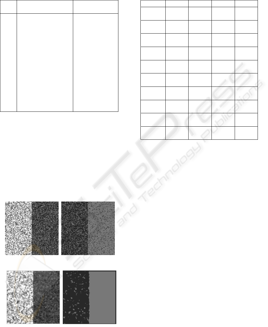
Table 4: Kurtosis.

α Kurtosis non-ﬁltered Kurtosis ﬁltered

images images

-1.5 81.5878 1.05008

-2.0 14.7974 0.797948

-2.5 9.90102 0.330502

-3.0 10.2707 0.229317

-3.5 7.36229 0.852436

-4.0 5.14167 0.117459

-4.5 3.10693 0.318509

-5.0 2.43030 0.145160

-5.5 2.35810 0.123555

-6.0 2.79451 0.297602

-6.5 1.93492 0.233789

-7.0 1.39388 0.328363

-7.5 1.66122 0.238216

-8.0 1.36633 0.299916

-8.5 0.998106 0.0621805

Table 5 shows the corresponding confusion matrix:

odd lines correspond to non-ﬁltered images and even

lines correspond to ﬁltered images. Data must be read

as follows: R

means the percentage of pixels that

belong to region R

but were classiﬁed into region R

and F

correspond to the non-ﬁltered image and

to the ﬁltered imge, respectively. From these values

it can be seen that the classiﬁcation performance was

better for ﬁltered images than for non- ﬁltered images.

(a) Original image (b) Image 7(a) classiﬁed

Figure 7: Synthetic, ﬁltered and classiﬁed images.

Table 5: Confusion matrix.

Imagen R

71.46 28.54 89.27 10.73

93.57 6.43 94.60 5.41

70.69 29.31 89.55 10.45

93.35 6.65 94.60 5.39

72.51 27.49 89.59 10.41

93.48 6.52 94.57 5.43

71.94 28.05 89.66 10.34

92.43 7.57 94.60 5.41

71.58 28.42 89.05 10.95

92.21 7.79 94.58 5.42

71.67 28.33 89.72 10.28

93.10 6.90 94.48 5.52

71.09 28.91 89.46 10.53

93.35 6.65 94.59 5.41

70.76 29.24 88.49 11.51

92.87 7.13 94.57 5.43

71.53 28.47 89.53 10.47

91.99 8.01 94.59 5.41

71.81 28.19 89.37 10.63

91.76 8.24 94.52 5.48

6 CONCLUSION

In this work, a study on the behaviour of adaptive

stack ﬁlters, applied to synthetic aperture radar (SAR)

images, was performed. The fundamentals of stack

ﬁlters were presented. These ﬁlters were applied to

simulated SAR images generated using the G

law

and were based on the algorithm proposed by (Yoo

et al., 1999). The statistical distribution of the ﬁl-

tered data was studied, and it was observed that they

no longer followed the above mentioned distribution.

We could infer that it turned out to be more similar

to the Gaussian distribution. Filtered and non-ﬁltered

images were classiﬁed according to the maximum

likelihood criterion. The classiﬁcation performance

was better for ﬁltered images than for non-ﬁltered im-

ages.

REFERENCES

Astola, J. and Kuosmanen, P. (1997). Fundamentals of Non-

linear Digital Filtering. CRC Press, Boca Raton.

Coyle, E. J., Lin, J.-H., and Gabbouj, M. (1989). Opti-

mal stack ﬁltering and the estimation and structural

approaches to image processing. IEEE Trans. Acoust.,

Speech, Signal Processing, 37:2037–2066.

Coyle, J. and Lin, J.-H. (1988). Stack ﬁlters and the mean

absolute error criterion. IEEE Trans. Acoust., Speech,

Signal Processing, 36:1244–1254.

ADAPTIVE STACK FILTERS IN SPECKLED IMAGERY

Frery, A. C., Correia, A. H., Renn

o, C. D., Freitas, C. C.,

Jacobo-Berlles, J., Mejail, M. E., and Vasconcellos,

K. L. P. (1999). Models for synthetic aperture radar

image analysis. Resenhas (IME-USP), 4(1):45–77.

Frery, A. C., M

uller, H.-J., Yanasse, C. C. F., and

Sant’Anna, S. J. S. (1996). A model for extremely het-

erogeneous clutter. IEEE Transactions on Geoscience

and Remote Sensing, 35(3):648–659.

Goodman, J. W. (1976). Some fundamental properties of

speckle. Journal of the Optical Society of America,

66:1145–1150.

J.Lin, H., M.Sellke, T., and J.Coyle, E. (1990). Adaptive

stack ﬁltering under the mean absolute error criterion.

IEEE Trans. Acoust., Speech, Signal Process, 38:938–

954.

Lin, J.-H. and Kim, Y. (1994). Fast algorithms for train-

ing stack ﬁlters. IEEE Trans. Signal Processing,

42(3):772–781.

Mejail, M. E. (1999). La Distribucin G

en el modelado

y Anlisis de Imgenes SAR. PhD thesis, Departamento

de Computacin, Facultad de Ciencias Exactas y Natu-

rales,Universidad de Buenos Aires.

Mejail, M. E., Frery, A. C., Jacobo-Berlles, J., and Bus-

tos, O. H. (2001). Approximation of distributions for

SAR images: proposal, evaluation and practical con-

sequences. Latin American Applied Research, 31:83–

92.

Mejail, M. E., Jacobo-Berlles, J., Frery, A. C., and Bustos,

O. H. (2003). Classiﬁcation of SAR images using a

general and tractable multiplicative model. Interna-

tional Journal of Remote Sensing, 24(18):3565–3582.

Oliver, C. and Quegan, S. (1998). Understanding synthetic

aperture radar images. Artech House.

Wendt, P., Coyle, E. J., and N.C. Gallangher, J. (1986).

Stack ﬁlters. IEEE Trans. Acoust. Speech Signal

Processing, 34:898–911.

Yoo, J., Fong, K. L., Huang, J.-J., Coyle, E. J., and III, G.

B. A. (1999). A fast algorithm for designing stack

ﬁlters. IEEE Trans.on image processing, 8(8):772–

781.

VISAPP 2006 - IMAGE FORMATION AND PROCESSING