HEAD ORIENTATION AND GAZE DETECTION FROM A SINGLE

IMAGE

Jeremy Yirmeyahu Kaminski

Computer Science Department, Holon Academic Institute of Technology,Holon, Israel

Adi Shavit and Dotan Knaan

Gentech Corporation, Israel Labs, Jerusalem, Israel

Mina Teicher

Bar-Ilan University,Ramat-Gan, Israel

Keywords:

Head Orientation, Gaze, Resultant.

Abstract:

Head orientation is an important part of many advanced human-machine interaction systems. We present a

single image based head pose computation algorithm. It is deduced from anthropometric data. This approach

allows us to use a single camera and requires no cooperation from the user. Using a single image avoids the

complexities associated with of a multi-camera system. Evaluation tests show that our approach is accurate,

fast and can be used in a variety of contexts. Application to gaze detection, with a working system, is also

demonstrated.

1 INTRODUCTION

Numerous systems need to compute head motion and

orientation. Instances are driver attention monitor-

ing and human-computer interface for multimedia or

medical purposes.

Therefore, for a large range of applications, the

need for a simple and efﬁcient algorithm for comput-

ing head orientation is crucial. Systems that must re-

cover at some stage some information on the 3D posi-

tion of the user’s head, run by deﬁnition in a complex

environment, because of the variety of human faces

and behaviors. That is the reason why, such a system

will gain in stability and usuability if the underlying

algorithm uses a simple setting. In that context, it is

worth noting that our algorithm is based on a single

camera and does not require from the user any cali-

bration.

Moreover, we shall present how our algorithm for

head orientation can be used for gaze detection too.

We describe an overall system, which performs gaze

detection from a single image. Our system turned out

to be accurate and fast, which makes it convenient for

a large variety of applications.

1.1 Comparison With Other

Approaches

Before introducing the core of our method, we present

a short comparison with previous works. Since the

problem of head position and gaze detection has re-

ceived a huge amount of attention in the past decade,

we do not pretend to establish a comprehensive re-

view of previous work. However we consider here-

after what seems to be the most relevant references to

show the novelty of our approach.

The large number of proposed algorithms for gaze

detection proves that no solution is completely satis-

fying. In (Glenstrup and Engell-Nielsen, 1995), one

can ﬁnd a good survey of several gaze detection tech-

niques. In (Ji and Yang, 2002; A.Perez, 2003), one

can ﬁnd a stereo system for gaze and face pose com-

putation, which is particularly suitable for monitor-

ing driver vigilance. Both systems are based on two

cameras, one being a narrow ﬁeld camera (which pro-

vides a high resolution image of the eyes by tracking

a small area) and the second being a large ﬁeld cam-

era (which tracks the whole face). Besides the com-

putationally complex difﬁculties arising from multi-

ple cameras and controlling these pan-tilt cameras,

the system hardware is quite costly. In (T. Ohno and

Yoshikawa, 2002), a monocular system is presented,

Yirmeyahu Kaminski J., Shavit A., Knaan D. and Teicher M. (2006).

HEAD ORIENTATION AND GAZE DETECTION FROM A SINGLE IMAGE.

In Proceedings of the First International Conference on Computer Vision Theory and Applications, pages 85-92

DOI: 10.5220/0001375800850092

 SciTePress

which uses a personal calibration process for each

user and does not allow large head motions. Limit-

ing the head motion is typical for systems that utilize

only a single camera. (T. Ohno and Yoshikawa, 2002)

uses a (motorized) auto-focus lens to estimate the dis-

tance of the face from the camera. In (J.G. Wang and

Venkateswarku, 2003), the eye gaze is computed by

using the fact that the iris contour, while being a cir-

cle in 3D is perspectively an ellipse in the image. The

drawback in this approach is that a high resolution im-

age of the iris area is necessary. This severely limits

the possible motions of the user, unless an additional

wide-angle camera is used.

In this paper we introduce a new approach with

several advantages. The system is monocular, hence

the difﬁculties associated with multiple cameras are

avoided. The camera parameters are maintained con-

stant in time. The system requires no personal cali-

bration and the head is allowed to move freely. This is

achieved by using a model of the face, deduced from

anthropometric features. This kind of method has al-

ready received some attention in past (T. Horprasert

and Davis, 1997; Gee and Cipolla, 1994a; Gee and

Cipolla, 1994b). However, our approach is simpler,

requires less points to be tracked and is eventually

more robust and practical.

In (Gee and Cipolla, 1994a; Gee and Cipolla,

1994b), the head orientation is estimated under the as-

sumption of the weak perspective image model. This

algorithm works using four points: the mouth cor-

ners and the external corners of the eyes. Once those

points are precisely detected, the head orientation is

computed by using the ratio of the lengths L

and L

where L

is the distance between the external eyes

corners and L

between the mouth and the eyes. In

(T. Horprasert and Davis, 1997), a ﬁve points algo-

rithm is proposed to recover the 3D orientation of

the head, under full perspective projection. The in-

ternal and external eyes corners provide four points,

while the ﬁfth point is the botton of the nose. The

ﬁrst four points approximately lie on a line. There-

fore the authors use the cross-ratio of these points as

a an algebraic constraint on the 3D orientation of the

head. It is worth noting that the cross-ratio is known

to be very sensitive to noise. Consider for exam-

ple, four points A, B, C, D lying on the x-axis which

x-coordinates are respectively 5, 10, 15, 20. These

points can be typically the eye corners. Then the

cross-ratio [A, B, C, D]=(5− 15)/(5− 20) × (10 −

20)/(10 − 15) = 10/3=3.333.NowifA is de-

tected at 4 and B at 11, then the cross-ratio becomes

[A, B, C, D]=(4− 15)/(5 − 20) × (11 − 20)/(11 −

15) = 99/64 = 1.54. This simple computation

shows that using the cross-ratio as a constraint on the

3D structure, requires detection with a precision gen-

erally beyond the capability of a vision system.

In contrast, our approach is based on three points

only and works with a full perspective model. The

three points are the eye centers and the middle point

between the nostrils. Using these three points, we can

compute several algebraic constraints on the 3D head

orientation, based on a anthropomorphic model of the

human face. These constraints are explicitly formu-

lated in section 2.

Once the head orientation is recovered, further

computations are possible. In this paper, we show an

application to gaze detection. This approach, of a me-

chanically simple, automatic and non-intrusive sys-

tem, allows eye-gazing to be used in a variety of ap-

plications where eye-gaze detection was not an option

before. For example, such a system may be installed

in mass produced cars. With the growing concern of

car accidents, customers and regulators are demand-

ing safer cars. Active sensors that may prevent acci-

dents are actively perused. A non-intrusive, cheaply

produced, one-size-ﬁts-all eye-gazing system could

monitor driver vigilance at all times. Drowsiness and

inattention can immediately generate alarms. In con-

junction with other active sensors, such as radar, ob-

stacle detection, etc. the driver may be warned of an

unnoticed hazard outside the car.

Psychophysical and psychological tests and exper-

iments with uncooperative subjects such as children

and/or primates, may also beneﬁt from such a static

(no moving parts) system, which allows the subject

to focus solely on the task at hand while remaining

oblivious to the eye-gaze system.

In conjunction with additional higher-level sys-

tems, a covert eye-gazing system may be useful in se-

curity applications. For example, monitoring the eye-

gaze of ATM clients. In automated airport checkin

counters, such a system may alert of suspiciously be-

having individuals.

The paper is organized as follows. In section 2,

we present the core of the paper, the face model that

we use and how this model leads to the computation

of the Euclidean face 3D orientation and position. We

present simulations, that show the results are robust to

error in both the model and the measurements. Sec-

tion 3 gives an overview of the system, and some ex-

periments are presented.

2 FACE MODEL AND

GEOMETRIC ANALYSIS

2.1 Face Model

Following the statistical data taken from (Farkas,

1994), we assume the following model of a generic

human face. Let A and B be the centers of the eyes,

and let C be the middle point between the nostrils.

VISAPP 2006 - IMAGE UNDERSTANDING

Figure 1: The face model is essentially based on the fact

that the triangle Eye-Nose Bottom-Eye is isosceles.

Then we assume the following model:

d(A, C)=d(B, C) (1)

d(A, B)=rd(A, C) (2)

d(A, B)=6.5cm (3)

where r =1.0833. The two ﬁrst equations allow

computing the orientation of the face, while the third

equation is necessary for computing the distance be-

tween the camera and the face. The face model is

illustrated in ﬁgure 1. The data gathered in (Farkas,

1994) shows that our model is widely valid over the

human population. Of course variations exist, but the

simulations presented in section 2.5 show that our al-

gorithm is quite robust over the whole spectrum of

human faces.

2.2 3D Face Orientation

Let M be the camera matrix. All the computations are

done in the coordinate system of the camera. There-

fore the camera matrix has the following expression:

M = K[I; 0],

where K is the matrix of internal parameters (Hartley

and Zisserman, 2000; Faugeras and Luong, 2001).

Let (a, b, c) be the projection of (A, B, C) onto

the image. In the equations below, the image points

a, b, c are given by their projective coordinates in the

image plane, while the 3D points A, B, C are given

by their Euclidean coordinates in R

. Given these no-

tations, the projection equations are:

a ∼ KA (4)

b ∼ KB (5)

c ∼ KC (6)

where ∼ means equality up to a scale factor. There-

fore the 3D points are given by the following expres-

sions:

A = αK

−1

a (7)

B = βK

−1

b (8)

C = γK

−1

c (9)

where α, β, γ are unknown scale factor. These could

also be deduced by considering the points at in-

ﬁnity of the optical rays generated by the image

points a, b, c and the camera center. These points

at inﬁnity are simply given in projective coordinates

by: [K

−1

a, 0]

, [K

−1

b, 0]

, [K

−1

c, 0]

. Then the

points A, B, C are given in projective coordinates by

[αK

−1

a, 1]

, [βK

−1

b, 1]

, [γK

−1

c, 1]

. These ex-

pressions naturally yield the equations (7), (8), (9)

giving the Euclidean coordinates of the points.

Plugging these expressions of A, B and C into the

two ﬁrst equations of the model (1) and (2), leads to

two homogeneous quadratic equations in α, β, γ:

f(α, β, γ)=0 (10)

g(α, β, γ)=0 (11)

Thus ﬁnding the points A, B and C is now reduced

in ﬁnding the intersection of two conics in the projec-

tive plane. Moreover since no solution is on the line

deﬁned by γ =0(since the nose of the user is not lo-

cated at the camera center!), one can reduce the com-

putation of the afﬁne piece deﬁned by γ =1. Hence

we shall now focus our attention on the following sys-

tem:

f(α, β, 1) = 0 (12)

g(α, β, 1) = 0 (13)

This system deﬁnes the intersection of two conics

in the afﬁne plane. The following subsection is de-

voted to the computation of the solutions of this sys-

tem.

2.3 Computing the Intersection of

Conics in the Afﬁne Plane

For sake of completeness, we shall recall shortly one

way of computing the solutions of the system above.

For more details, see (Sturmfels, 2002). Consider ﬁrst

two polynomials f, g ∈ C[x]. The resultant gives a

way to know if the two polynomials have a common

root. Write the polynomials as follows:



f = a

+ ... + a

x + a

g = b

+ ... + b

x + b

The resultant of f and g is a polynomial r, which

is a combination of monomials in {a

}

i=1,...,n

and

}

j=1,...,p

with coefﬁcients in Z, that is r ∈

Z[a

]. The resultant r vanishes if and only if either

or b

is zero or the polynomials have a common

root in C. The resultant can be computed as the de-

terminant of a polynomial matrix. There exist several

matrices whose determinant is equal to the resultant.

The best known and simplest matrix is the so-called

HEAD ORIENTATION AND GAZE DETECTION FROM A SINGLE IMAGE

Sylvester matrix, deﬁned as follows:

S(f,g)=

⎡

⎢

⎣

00... 0 b

00... 0

n−1

0 ... 0 b

p−1

0 ... 0

. .

⎤

⎥

⎦

Therefore, we have:

r(x)=det(Syl(f, g)).

In addition to this expression which gives a practical

way to compute the resultant, there exists another for-

mula of theoretical interest:

r(x)=a

α,β

− x

where x

are the roots of f and x

are those of g.

It can be shown that the resultant is a polynomial of

degree np.

An important point is that the resultant is also de-

ﬁned and has the same properties if the coefﬁcients of

the polynomials are not only numbers but also poly-

nomials in another variable. Hence, consider now that

f,g ∈ C[x, y] and write:



f = a

(x)y

+ ... + a

(x)y + a

(x)

g = b

(x)y

+ ... + b

(x)y + b

(x)

(14)

The question is now the following: given a value x

of x, do the two polynomials f(x

,y) and g(x

,y)

have a common root? The answer to this question is

based on the computation of the resultant of f and

g with respect to y (i.e. using the presentation given

by (14)). This is a univariate polynomial in x, denoted

by r(x)=res(f,g,y).

The resultant can be used in many contexts. For

our purpose, we will use it to compute the intersec-

tion points of two planar algebraic curves. Consider

the curve C

(respectively C

) deﬁned as the set of

points (x, y) which are roots of f(x, y) (respectively

g(x, y)). We want to compute the intersection of C

and C

. Algebraically, this is equivalent to computing

the common roots of f and g. Therefore, we use the

following procedure:

• Compute the resultant r(x)=res(f,g,y) ∈ C[x].

• Find the roots of r(x): x

, ..., x

• For each i =1, ..., t, compute the common roots of

f(x

,y) and g(x

,y) in C[y]: y

, ..., y

• The intersection of C

and C

is therefore:

), ..., (x

In our context, the resultant r is polynomial of de-

gree 4 and so t ≤ 4 and k

≤ 2. To complete the pic-

ture, we just need to mention an efﬁcient and reliable

way to compute the roots of a univariate polynomial.

The algorithm that we will describe is very efﬁcient

and robust for low degree polynomials. Given a uni-

variate polynomial p(x)=a

+... +a

x+ a

, one

can form the following matrix, called the companion

matrix of p:

C(p)=

010... 0

001... 0

−a

... −a

n−1

A short computation shows that the characteristic

polynomial of C(p) is equal to −

p. Thus the roots

of p are exactly the eigenvalues of C(p). This pro-

vides one practical way to compute the roots of a uni-

variate polynomial.

2.4 3D Face Orientation

Therefore, we solve the system S deﬁned by equa-

tions (12) and (13) using the approach presented

above. By Bezout’s theorem (or simply by looking

at the degree of the resultant), we know that there are

at most 4 complex solutions to this system. Experi-

ments show that a system generated by the image of

a human face has only two real roots. The ambiguity

between these two roots is easily handled, since one

solution leads to non realistic eye-to-eye distance. Let

(α

,β

) be the right solution. Then the points A, B

and C are known up to a unique scale factor. We shall

denote A

, B

and C

the points obtained by the so-

lution (α

,β

), Thus we have the following expres-

sion:

= α

−1

a (15)

= β

−1

b (16)

= K

−1

c (17)

Thus we have the following relations too: A = γA

B = γB

and C = γC

The computation of γ is done using the third model

equation (3). Once the face points are computed, we

can compute the distance between the user’s face and

the camera and so the 3D orientation of the face. In-

deed the normal to the plane deﬁned by A, B and C

is given by:

−→

N =

−−→

AB ∧

−→

AC,

where ∧ is the cross product.

2.5 Robustness to Errors in Model

and Detection

In order to estimate the sensitivity of this algorithm to

errors in model and in detection, we performed sev-

eral simulations. As we shall detail in subsection 3.1,

we use a rather high resolution camera. Therefore in

the simulation, we start from the following setting:

VISAPP 2006 - IMAGE UNDERSTANDING

0.2

0.4

0.6

0.8

1.2

3D Reconstruction Error (cm)

20 40 60 80 100

Noise Standard Deviation

Figure 2: Inﬂuence of the error in focal length.

• The focal length f = 4000 in pixels (which is very

close to the value of the actual camera used in the

system),

• The principal point is at the image center,

• The distance between the camera and the face is

60cm (which is the actual setting of the system).

The simulations are done according to the follow-

ing protocol. An artiﬁcial face, deﬁned by three points

in space, say A, B and C, is projected onto a known

camera. Given a parameter p, we perform a perturba-

tion of p by a white Gaussian noise of standard devi-

ation σ. For each value of σ, we perform 100 random

perturbations. For each value of p, obtained by this

process, we compute the error in the 3D reconstruc-

tion as the mean of the square errors.

The ﬁrst simulation (see ﬁgure 2) shows that the

system is very robust to errors in the estimation of the

focal length, since for a noise with standard deviation

of 100 (in pixels), the reconstruction error is 1.2cm,

less than 1% of the distance between the camera and

the user.

The next two simulation aim at measuring the inﬂu-

ence of errors in model. First, the assumed eye-to-eye

distance is corrupted by a Gaussian white noise (ﬁg-

ure 3). The mean value is 6.5cm as mentioned in sec-

tion 2. For a standard deviation of 0.5, which repre-

sents an extreme anomaly with respect to the standard

human morphology, the reconstruction error is about

3.3cm, less than 2% of the distance between the cam-

era and the user. The inﬂuence of the human ratio

r, as deﬁned in equation (2), is also tested by adding

a Gaussian white noise, centered at the ”universal”

value 1.0833 (ﬁgure 4). For a standard deviation 0.15,

which also represents a very strong anomaly, the re-

construction is 1.75cm, just over 1% of the distance

between the camera and the user.

After measuring the inﬂuence of errors in camera

calibration and model, the next step is to evaluate

the sensitivity to input data perturbation. The image

1.5

2.5

3D Reconstruction Error (cm)

0.1 0.2 0.3 0.4 0.5

Noise Standard Deviation

Figure 3: Inﬂuence of the error in inter-eyes distance.

0.2

0.4

0.6

0.8

1.2

1.4

1.6

3D Reconstruction Error (cm)

0.02 0.04 0.06 0.08 0.1 0.12 0.14

Noise Standard Deviation

Figure 4: Inﬂuence of the error in human ratio.

0.2

0.4

0.6

0.8

1.2

1.4

1.6

1.8

3D Reconstruction Error (cm)

246810

Noise Standard Deviation

Figure 5: Inﬂuence of the error in image points.

points are corrupted by a Gaussian white noise (ﬁg-

ure 5). For a noise of 10 pixels, which is a large er-

ror in detection, the reconstruction error is less 2cm,

about 1.15% of the distance between the camera and

the user.

HEAD ORIENTATION AND GAZE DETECTION FROM A SINGLE IMAGE

The accuracy of the system is mainly due to the fact

that the focal length is high (f = 4000 in pixels). In-

deed when computing the optical rays generated by

the image points, as in equations (7,8,9), we use the

inverse of K, which is roughly equivalent to multiply-

ing the image points coordinates by 1/f . Hence the

larger f is, the less impact a detection error has on the

computation.

3 APPLICATION: GAZE

DETECTION SYSTEM

In this section, we show how the ideas presented

above can be used to build a gaze detection system,

that does not require any user calibration or interac-

tion.

3.1 System Architecture

The main practical goal of this work was to create a

non-intrusive gaze detection system, that would re-

quire no user cooperation while keeping the system

complexity low. We use a high-resolution 15 fps,

1392x1040 video camera with a 25mm ﬁxed-focus

lens. The CCD pixel is a square of length equal to

6.45 microns. Thus the focal length is 3875, which

is the same order of magnitude as the value used in

the simulation. This setup allows both a wide ﬁeld of

view, for a broad range of head positions, and high

resolution images of the eyes. Since we can estimate

the 3D head position from a single image, we can use

a ﬁxed focus lens instead of a motorized auto-focus

lens. This makes the camera calibration simpler and

the calibration of the internal parameters is done only

once. The system uses an IR LED at a known position

to illuminate the user’s face.

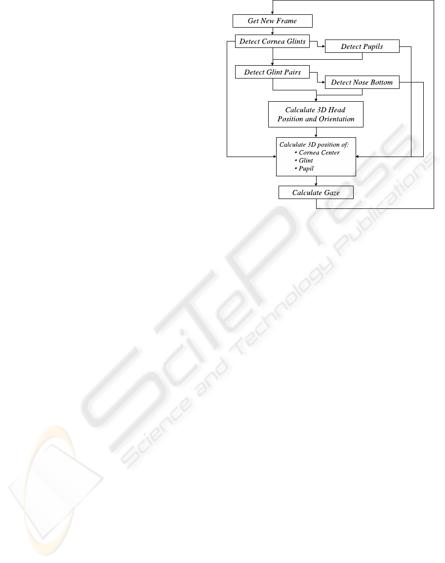
3.2 System Overview

The general ﬂow of the system is depicted in Figure 6.

For every new frame, the glints, that is the reﬂections

of the LED light from the eye corneas as seen by the

camera, are detected and their corresponding pupils

are found. The search area for the nose is then de-

ﬁned, and the nose bottom is found. Given the two

glints and nose position, we can reconstruct the com-

plete Euclidean 3D face position and orientation rel-

ative to the camera, using the geometric algorithm

presented in section 2. This reconstruction gives us

the exact 3D position of the glints and pupils. Then,

for each eye, the 3D cornea center is computed us-

ing the knowledge of LED position, as shown in ﬁg-

ure 8. This model is similar to the eye model used

in (T. Ohno and Yoshikawa, 2002). The following

Figure 6: The system ﬂow chart, showing the different

stages of the process.

sub-sections 3.3 and 3.4 will describe these stages in

more detail.

3.3 Feature Detection

3.3.1 Glint and Pupil Detection

The detection of the glints is done in several steps.

Glints appear as very bright dots in the image, usu-

ally at the highest possible grayscale values. Us-

ing a thresholding operation on the image yields

multiple candidates for possible glints. Examples

of other sources of similar characteristics are back-

ground lights, facial hair, teeth and lenses and frames

of eye-glasses. We perform multiple ﬁltering stages

to identify the true glints. We ﬁlter these candidates

by size, i.e. we select only the small dot-like ones.

Next, we pair-up the remaining candidates and select

only those glint-pairs that satisfy certain constraints

on distances and angles.

We next proceed to the detection of the pupils. The

pupils serve two purposes. They are used to ﬁlter out

incorrect glint pairs, and they are required for the cal-

culation of the gaze direction in the later stages of the

algorithm. Pupils appear as round or oval dark regions

inside the eye and are very close to (or behind) the

glints. We search for these dark regions around each

of our detected glints. Glint pairs containing a glint

around which no pupil was found are removed. This

ﬁnal glint ﬁltering will usually leave us with the ﬁ-

nal true glint pair. Otherwise, we choose the top-most

pair, as empirically, it was shown to be the correct

one.

VISAPP 2006 - IMAGE UNDERSTANDING

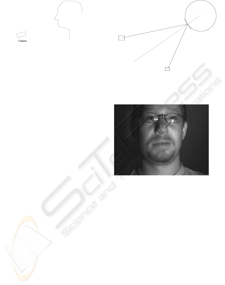
Figure 7: The camera is viewing the eyes and the nostrils.

3.3.2 Nose Detection

The detection of the nose-bottom is done by searching

for dark-bright-dark patterns in the area just below the

eyes. Indeed, the nostrils appear as dark blobs in the

image thanks to the relative position of the camera and

the face as shown in ﬁgure 7. The size and orientation

of this search area is determined by the distance and

orientation of the chosen glint-pair. Once dark-bright-

dark patterns are found, we use connected component

blob analysis on this region to identify only those dark

blobs that obey certain size, shape, distance and rela-

tive angle constraints that yield plausible nostrils. The

nose bottom is selected as the point just between the

two nostrils.

3.4 Gaze Detection

Given the glints and the bottom point of the nose, one

can apply the geometric algorithm presented in sec-

tion 2 to compute the 3D face orientation. As seen in

subsection 2.5, even if the glints are not exactly lo-

cated in the center of the eye, the system returns an

accurate answer. Then for each eye, the cornea center

is computed using the knowledge of LED position, as

shown in ﬁgure 8.

The gaze line is deﬁned as being the line joining

the cornea center and the pupil center in 3D.

The pupil center is ﬁrst detected in the image and

computed in 3D as follows. The distance between the

pupil center and the cornea center is a known measure

of the human anatomy. It is equal to 0.45 cm. Con-

sider then a sphere S centered at the cornea center,

with radius equal to 0.45 cm. The pupil center lies

on the optical ray generated by its projection onto the

image and the camera center. This ray intersects the

sphere S in two points. The closest of these points to

the camera is the pupil center.

4 EXPERIMENTS

We show sample images produced by the system,

where one can see the detected triangle, deﬁned by

Cornea

Center

amera

LED

Glint in 3D

Figure 8: The cornea center lies on the bisector of the angle

deﬁned by the LED, the glint point in 3D and the camera.

Its exact location is given by the cornea radius, which is

77mm.

Figure 9: The detected triangle, eyes’ centers and the nose

bottom, together with the gaze line.

the eyes’ centers and the bottom points of the nose.

In addition, the gaze line is reprojected onto the im-

ages and rendered by white or blacks arrows, ﬁgure 9,

10, 11.

5 DISCUSSION

We proposed an automatic, non-intrusive eye-gaze

system. It uses an anthropomorphic model of the hu-

man face to calculate the face distance, orientation

and gaze angle, without requiring any user-speciﬁc

calibration. This generality, as seen in subsection 2.5,

does not introduce large errors into the gaze direction

computation. A patent application (number in Japan:

2005-253778) has been led covering the geometric as-

pects and the features detection.

While the beneﬁts of a calibration-free system al-

low for a broad range of previously impossible appli-

cations, the system design allows for easy plugging of

HEAD ORIENTATION AND GAZE DETECTION FROM A SINGLE IMAGE

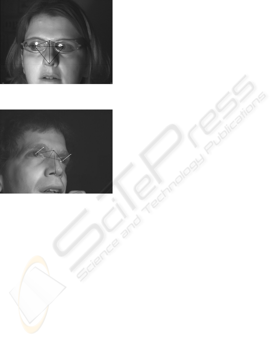
Figure 10: The detected triangle, eyes’ centers and the nose

bottom, together with the gaze line.

Figure 11: The detected triangle, eyes’ centers and the nose

bottom, together with the gaze line.

user-speciﬁc calibration data, which will increase the

accuracy even more.

REFERENCES

A.Perez, M.L. Cordoba, A. Garcia, R. Mendez, M.L.

Munoz, J.L. Pedraza and F. Sanchez (2003) A pre-

cise eye-gaze detection and tracking system. In 11th

International Conference in Central Europe on Com-

puter Graphics, Visualization and Computer Vision.

Farkas, L. (1994). Anthropometry of the Head and Face.

Raven Press.

Faugeras, O. and Luong, Q. (2001). The Geometry of Mul-

tiple Images. MIT Press.

Gee, A. and Cipolla, R. (1994a). Estimating gaze from a

single view of a face. In IAPR 12th International Con-

ference on Pattern Recognition.

Gee, A. and Cipolla, R. (1994b). Non-intrusive gaze track-

ing for human-computer interaction. In International

Conference on Mechatronics and Machine Vision in

Practice.

Glenstrup, A. and Engell-Nielsen, T. (1995). Eye Con-

trolled Media: Present and Future State. University

of Copenhagen, DK-2100.

Hartley, R. and Zisserman, A. (2000). Multiple-view Geom-

etry. Cambrigde University Press.

J.G. Wang, E. S. and Venkateswarku, R. (2003). Eye gaze

estimation from a single image of one eye. In 9th

IEEE International Conference on Computer Vision.

Ji, Q. and Yang, X. (2002). Real-time eye, gaze, and face

pose tracking for monitoring driver vigilance. In Real-

Time Imaging, 8, 357-377.

Sturmfels, B. (2002). Solving Systems of Polynomial Equa-

tions. American Mathematical Society.

T. Horprasert, Y. Y. and Davis, L. (May 1997). An anthro-

pometric shape model for estimating head orientation.

In 3rd International Workshop on Visual Form, Capri,

Italy.

T. Ohno, N. M. and Yoshikawa, A. (2002). Freegaze: A

gaze tracking system for everyday gaze interaction. In

Symposium on Eye Tracking Research and Applica-

tions.

VISAPP 2006 - IMAGE UNDERSTANDING