
AN EFFICIENT CATADIOPTRIC SENSOR CALIBRATION BASED
ON A LOW-COST TEST-PATTERN
N. Ragot
Institut de Recherche en Systèmes Electroniques EMbarqués
Technopôle du Madrillet - Avenue Galilée - BP 10024, 76801 St Etienne du Rouvray, France
J. Y. Ertaud, X. Savatier, B. Mazari
Institut de Recherche en Systèmes Electroniques EMbarqués
Technopôle du Madrillet - Avenue Galilée - BP 10024, 76801 St Etienne du Rouvray, France
Keywords:
Panoramic vision, catadioptric sensor, stereovision, calibration.
Abstract:
This article presents an innovative calibration method for a panoramic vision sensor which is dedicated to the
three-dimensional reconstruction of an environment with no prior knowledge. We begin this paper by a de-
tailed presentation of the architecture of the sensor. We mention the general features about central catadioptric
sensors and we clarify the fixed viewpoint constraint. Next, a large description of the previous panoramic
calibration techniques is given. We mention the different postulates which lead us to envisage the method of
calibration presented in this paper. A description of the low-cost calibration test pattern is given. The algo-
rithmic approach developed is detailed. We present the results obtained. Finally, the last part is devoted to the
result reviewing.
1 INTRODUCTION
Within the framework of applications where the sen-
sor is mobile and where there is no prior knowledge of
the environment (no cartographic models available),
the knowledge of the exact spatial localization of the
sensor is necessary to make a reliable 3D reconstruc-
tion. This is known as the paradigm of localization
and dynamic environmental modelling (C. Drocourt
and Cauchois, 2001). Thus, two kinds of sensors are
employed. The first ones are called proprioceptive
sensors and are used to provide the mobile with data
on its intrinsic state. The second ones are called exte-
roceptive sensors and are used to provide information
to the mobile about the external environment in which
it moves. The ignorance of the environmental charac-
teristics impose to the ideal exteroceptive sensor to
provide the most complete and precise 3D represen-
tation of the environment. This information coupled
the proprioceptive sensor data allows a reliable inter-
pretation of the observed environment.
3D exteroceptive perception systems can be classi-
fied in different categories (Nitzan 1988). Majority
of them are reliable but can not render a wide zone
instantaneously. Vision systems and their ability to
acquire in a one-shot image all of the information of
a volume of a given space has been investigated. This
volume, defined by the aperture of the camera, can
be increased artificially by combining views given by
multiple or rotating cameras (T. Ea and Garda, 2001).
Another method consists in coupling a mirror with
a camera (S. Baker, 2001), (Zhu, 2001). These are
known as catadioptric systems and images obtained
are panoramic views of the environment (C. Geyer,
2001).
The architecture of the sensor presented in this pa-
per offers a solution to the problem of 3D percep-
tion of an environment with no prior knowledge. This
sensor is a panoramic stereovision system constituted
of two catadioptric vision sensors. The main objec-
tive of this article is to present an innovative cali-
bration which is the preliminary step to the elabora-
tion of a three-dimensional reconstruction. We begin
by a detailed presentation of the sensor architecture.
We give some general features about catadioptric sen-
sors and we highlight the fixed viewpoint constraint
which is presented as the main requirement to process
pure perspective images. We refer to calibration tech-
niques for panoramic vision sensors. We detail the
proposed calibration principles and we give a large
description of the test pattern used. We show the re-
sults obtained and we provide a critic analysis about
their viability. The last part summarizes the different
reflections leaded and gives some work perspectives.
11
Ragot N., Y. Ertaud J., Savatier X. and Mazari B. (2006).
AN EFFICIENT CATADIOPTRIC SENSOR CALIBRATION BASED ON A LOW-COST TEST-PATTERN.
In Proceedings of the First International Conference on Computer Vision Theory and Applications, pages 11-18
DOI: 10.5220/0001374100110018
Copyright
c
SciTePress
2 ARCHITECTURE OF THE
STEREOVISION PANORAMIC
SENSOR
The proposed innovative architecture offers a solution
to the problem of 3D perception of an environment
with no prior knowledge. The main objective of the
study is to develop an exteroceptive stereovision sen-
sor which enables a vision and the most complete 3D
reconstruction of the environment. This exteroceptive
sensor is made of two catadioptric vision systems.
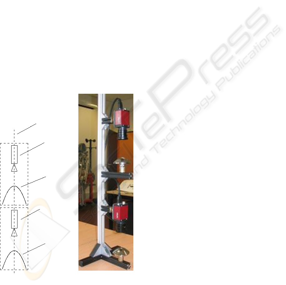
Each of the catadioptric sensor is composed of a
hyperboloid mirror H3S from Neovision coupled with
a classic Marlin-F-145C perspective camera from Al-
lied Vision with a 6.5mm focal length. The elements
are fixed vertically with their optical axis in common
(cf. Figure 1). As a result, the mathematical equa-
tions are simplified. Moreover, it enables the simplifi-
cation of the epipolar relation associating the two om-
nidirectional sensors. Lastly, it enables the detection
of horizontal primitives which is favoured within the
framework of our applications.
High camera
in common
Optical axis
Low camera
mirror
High hyperboloid
Low hyperboloid
mirror
Figure 1: Architecture of the panoramic stereovision sensor.
Left: Schema of a cross-section view of the sensor. Right:
Image of the sensor developed.
3 CATADIOPTRIC SENSOR:
GENERAL FEATURES AND
PREVIOUS CALIBRATION
WORKS
3.1 General Features
Catadioptric sensors are powerful due to their
panoramic vision. Nevertheless, coupling the conven-
tional projective linear model (which enables a pure
perspective image formation) to mirror equations can
only be done with respect to the fixed viewpoint con-
straint (Svoboda, 1999). In such a case, the vision
system is called a central catadioptric sensor and a
geometrically pure perspective image is formed. Two
main points have to be mentioned. First, the effec-
tive pinhole which is intrinsic to the pinhole model,
is also called the principal point of the camera. Sec-
ond, the effective viewpoint which is intrinsic to the
mirror is defined as the focus of the mirror. The fixed
viewpoint constraint, also called the single effective
viewpoint constraint, is defined as the requirement
that vision systems only measure the intensity of light
passing through a single 3D point. Work made by
Baker et al. (S. Baker, 1999) consists in the deriva-
tion of the fixed viewpoint constraint equation. They
deduce from the obtained results several types of mir-
rors respecting this constraint (e.g. ellipsoidal, hy-
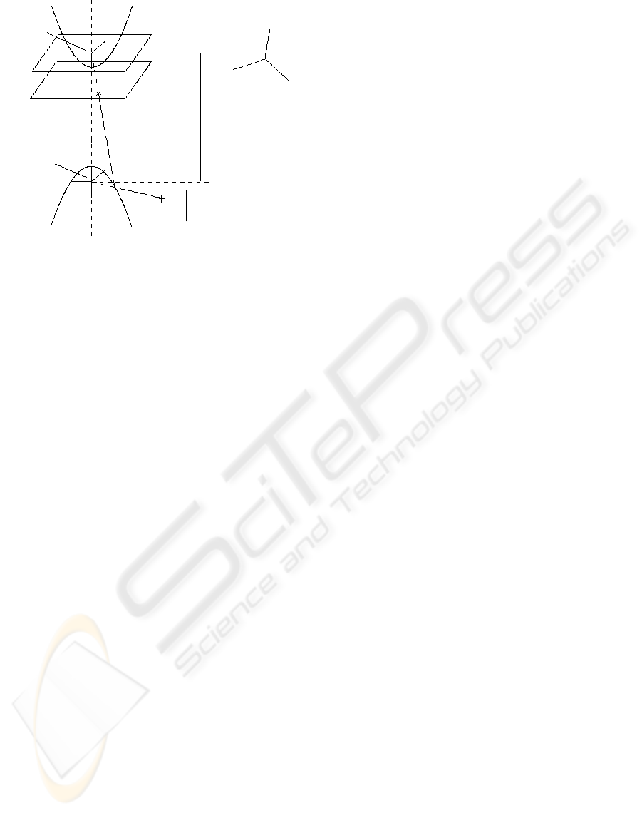
perboloidal mirrors). The figure above (cf. Figure 2)
illustrates the fixed viewpoint constraint in the case
of an hyperboloid mirror. The rays of light coming
from a 3D point which seem to meet at the effective
viewpoint are reflected by the shape of the mirror and
converge at the effective pinhole.
3.2 Previous Calibration Works
The calibration enables to match 3D points in the
world frame to 2D pixels in the image planes. Differ-
ent types of techniques enable to calibrate a catadiop-
tric vision system. The description and classification
given below is greatly inspired from the work of El
Mouaddib (Mouaddib, 2005).
• The intrinsic calibration consists in the establish-
ment of the intrinsic parameters. In the case of
catadioptric sensors, the parameters to be estimated
are related to the mirror, lens, CCD matrix and the
video acquisition board. This method consists in
the exploitation of the mirror imprint on the image
and the mirror data dimensions given by the manu-
facturer. The work made by Fabrizio et al. (J. Fab-
rizio, 2002) is a significant example of this tech-
nique. The principle is to exploit the boundaries of
the mirror as a calibration pattern. This technique
is powerful due to the missing calibration pattern.
VISAPP 2006 - IMAGE FORMATION AND PROCESSING
12
/
?
>
>
?
P
w
Z
w
X
w
Y
w
v
u
Z
w
X
w
Y
w
)
R
Focal plane
Image plane
Mirror frame
Camera frame
6
?
Eccentricity
Real sheet of the hyperboloid
Virtual sheet of the hyperboloid
World frame
Retinal frame
j
j
6
Figure 2: Illustration of the fixed viewpoint constraint in the
case of a hyperboloid mirror. The focus of the virtual sheet
corresponds to the principal point of the camera (the focus
of the camera). The distance between the two foci is called
the eccentricity.
Nevertheless it requires the prior knowledge of the
geometric mirror characteristics.
• The self-calibration is based on the same principles
as for the classical cameras. It consists in the es-
tablishment of the fundamental and essential ma-
trices. Thus, it requires a minimum of two image
planes and the pixel matching. The pixel matching
is based on certain constraints such as uniqueness,
ordering, orientation, continuity, disparity gradient.
The epipolar constraint is the most powerful one
(Faugeras, 1993). We can mention the work of
Svoboda et al. (T. Svoboda, 1998) which estab-
lishes the epipolar geometry for central panoramic
cameras using hyperboloid mirrors. The signifi-
cant works for catadioptric self-calibration are the
one made by Kang (Kang, 2000) and Mariottini
(G.L. Mariottini, 2005). The first one is based on
the derivation of the epipolar relation for catadiop-
tric sensors made of paraboloid mirrors and cali-
brate the stereovision panoramic system. The sec-
ond one is a powerful tool developed under MAT-
LAB environment which enables the determina-
tion of the epipolar matrices for classical and/or
panoramic stereovision sensors.
• The most common method is the one exploiting
an external test pattern. This technique is based
on the exact knowledge of geometrical figure co-
ordinates (generally points) forming the calibration
tool, expressed in a local frame and their 2D match-
ings. For a sufficient number of matching, an op-
timization algorithm is applied (e.g. Levenberg-
Marquardt (L. Smadja, 2004), (Lacroix et al.,
2005)). This method is powerful because it is ap-
plicable to all type of catadioptric sensor. More-
over, it enables the estimation of intrinsic and ex-
trinsic parameters. The high number of parameters
to be estimated requires a high care for the conver-
gence initialization of the optimization algorithm.
One of the significant work is made by Cauchois et
al. (C. Cauchois and Clerentin, 1999). It exploits
a catadioptric sensor formed by a conical mirror.
The calibration exploits two type of two plane cal-
ibration pattern. One is placed on the top of the
cone. The other is perpendicular and enables the
estimation of all parameters. The work made by
Moldovan (Moldovan, 2004) exploits a cylindri-
cal test pattern formed by a large number of LED
which locations are perfectly known. The work
made by Ying et al. (X. Ying, 2003) is based on the
theory of the invariants and exploits the projection
of lines and spheres. As well, we can mention the
work of Barreto et al. (J.P. Barreto, 2005) which
demonstrates that three lines are sufficient for the
calibration of all central catadioptric sensor.
As well, this calibration technique is used for ap-
plications of active omnidirectional stereovision.
We can mention the work made by Marzani et
al. (F. Marzani and Voon, 2002) which exploits a
catadioptric sensor coupled with a laser diode. A
bitmap beam is projected on a plane which stands
for the external calibration pattern.
4 CALIBRATION PROPOSED
4.1 Postulates
The calibration proposed stems from two postulates:
• The optics (mirrors and lens) are imperfect by na-
ture. Impurities and defaults can not be avoided
despite the great precautions taken during the prod-
uct design (Moldovan, 2004). These imperfections
imply local distortions which are difficult to model
and thus to take into account.
• The single effective viewpoint constraint is particu-
larly difficult to realize in hardware implementation
(Aliaga, 2001).
The calibration exposed intends to establish 3D/2D
matchings, the vision sensor being considered as a
"black box". This enables to break of the problems
listed previously. This calibration method presented
can be considered as a generalization of the one de-
veloped by Biber et al. (P. Biber and Andreas, 2004).
4.2 Method
A catadioptric system provides a circular image of the
environment. A pixel, or a sub-pixel p is defined by
AN EFFICIENT CATADIOPTRIC SENSOR CALIBRATION BASED ON A LOW-COST TEST-PATTERN
13
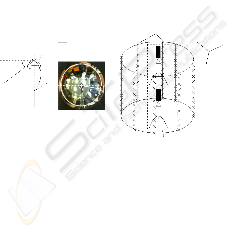
its azimut angle α (0<α<360 degrees) and its radius
r (cf. Figures 3, 7). α defines the horizontal posi-
tion of the 3D point P
M
(X
M
,Y
M
,Z
M
) and thus is
linked to its coordinates X
M
, Y
M
. In the same way
the euclidian distance r defines the vertical position of
the 3D point and thus is linked to the coordinate Z
M
.
Moreover, r can be associated to the angle γ which
is defined as the angle from the axis passing through
the focus of the mirror and parallel to the axis X
M
to
the 3D point. The range in which γ lies tightly de-
pends on the mirror geometry. This specification is
generally provided by the manufacturer. In our con-
figuration γ lies from −15 to 90 degrees. Finally, γ
is linked to the 3D point coordinates and can be ex-
pressed as follows (1). The Figure above elaborates
the matching between a 3D point to a pixel (cf. Fig-
ure 3):
tan γ =
Z
M
X
M
(1)
?
3
γ
X
M
Y
M
Z
M
Z
M
X
M
Y
M
P
M
Hyperboloid mirror
I
Mirror frame
O
Figure 3: Illustration of the relation linking a 3D point to
the pixel radius r. (Right: O stands for image centre, p for
pixel position and α for the azimut angle).
Like this, the 3D/2D matching depends on vari-
ables α and r. It can be defined as follows:
∃f | γ = f (α, r)
4.3 Implementation
The 360 degrees field of view and the 2D spherical co-
ordinates of a pixel or a sub-pixel lead to design and
use a cylindrical test pattern. This form is inspired
from the works of Moldovan (Moldovan, 2004). The
test pattern used is a low-cost one an it is made of rigid
PVC. Its height is 1400mm and the internal diameter
is 595mm (the thickness of the cylinder is 5mm). This
test pattern is formed by a large number of white LED
which 3D cartesian coordinates are perfectly known
in the frame of the calibration tool. They are verti-
cally arranged with a regular interval. The horizon-
tal angle between each LED is constant (45 degrees).
The choice of white color markers is voluntary for two
reasons. First, the contrast between the darkness in-
side the tube and the LED is pronounced. Second,
the white light codes the totality of the RGB compo-
nents which up the sensitivity. Moreover, the angle
of diffusion as well as the light intensity are parame-
ters which are particularly be examined. The angle of
diffusion is 70 degrees. It is 2.5 times up than for a
classical LED. The light intensity is 1190mcd, which
is approximately 4 times up than for a common LED.
These characteristic enable the obtaining of signifi-
cant spot lights on each CCD. Next, the sensor is in-
serted into this test pattern (cf. Figure 4). A particular
attention is provided to make sure that the optical axis
is aligned with the center of the test pattern.
O
inserted into the test pattern
Catadioptric stereovision sensor
Test pattern formed by a large number of LED
R
World frame
*
}
X
w
Z
w
Y
w
Figure 4: Illustration of the test pattern used to manage the
calibration step.
A segmentation algorithm using a local recursion is
applied to the two images which enables to reference
the markers identified as areas coverage. This local
segmentation is done following a criterion of simi-
larity between a reference pixel (p
r
) and the pixel in
reading (p
i
). This criterion is based on the estima-
tion of the color difference by the determination of
the euclidean distance. Then, a research of the centre
of gravity coordinates is applied to each spot light.
This enables to know their exact sub-pixel coordi-
nates. Finally, the 3D points coordinates, the α angle
and the euclidean distance r being known, the func-
tion γ = f (α, r) can be established (cf. Figure 5).
VISAPP 2006 - IMAGE FORMATION AND PROCESSING
14
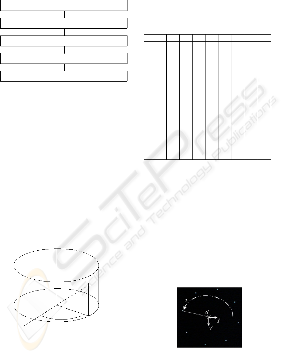
Image acquisition of the calibration external pattern
Segmentation using a local recursion
Determination of the barycentre of each area coverage
γ = f(α, r)
Bilinear interpolation
?
?
?
?
Figure 5: The block diagram describing the calibration
process.
5 RESULTS
The markers are referenced in a cartesian frame
(O, X
TP
,Y
TP
,Z
TP
), which is located at the bottom
centre of the cylinder (cf. Figure 6). They are ex-
pressed in cylindrical coordinates and are summa-
rized in the table (cf. Table 1). The positioning of
the markers implies that for each LED Bar Bi, the
parameter h
i
defined as the vertical component, is the
single one variable.
The particular configuration, in which Z
TP
axis is
merged with the optical axis of the sensor, enables an
immediate expression of the coordinates of the mark-
ers in each mirror frame. Thus, the angle γ which is
linked to the position of the markers and expressed in
each mirror frame can be easily determined. More-
over, for points located at a same altitude, the angle γ
is equivalent.
O
-
6
+
θ
6
q
1
X
TP
Y
TP
Z
TP
P
R
h
Figure 6: Localisation of the frame of the test-pattern.
The image acquisitions are carried out so that the
eight markers located at a same altitude, are lighted
simultaneously (cf. Figure 7). As mentioned pre-
viously, simple image processings permit the de-
termination of homogenous regions and all mark-
Table 1: Cylindrical coordinates of the markers. Bi stands
for LED Bar. Considering each LED bar separately, h
i
is the only variable parameter following the vertical axis
(Z
TP
).
B1 B2 B3 B4 B5 B6 B7 B8
Radius R
(mm)
289.5 289.5 289.5 289.5 289.5 289.5 289.5 289.5
θ
(degrees)
0 45 90 135 180 225 270 315
h
1
50 50 50 50 50 50 50 50
h
2
150 150 150 150 150 150 150 150
h
3
250 250 250 250 250 250 250 250
h
4
350 350 350 350 350 350 350 350
h
5
450 450 450 450 450 450 450 450
h
6
550 550 550 550 550 550 550 550
h
7
650 650 650 650 650 650 650 650
h
8
750 750 750 750 750 750 750 750
h
9
850 850 850 850 850 850 850 850
h
10
950 950 950 950 950 950 950 950
h
11
1050 1050 1050 1050 1050 1050 1050 1050
h
12
1150 1150 1150 1150 1150 1150 1150 1150
h
13
1250 1250 1250 1250 1250 1250 1250 1250
h
14
1350 1350 1350 1350 1350 1350 1350 1350
ers barycentre localisation. Thus, the determination
of pixel or sub-pixel polar coordinates (r,α) are ob-
tained. These two parameters are expressed in a local
image frame (O
,u
,v
) which the point O
is located
at the centre of the images and the axes (u
,v
) are
parallel to those of the retinal plane (u, v). The results
are summarized on the four next tables. The tables
above (cf. Tables 2, 3) describe the results obtained
for the low sensor and the next ones (cf. Tables 4, 5)
those obtained for the high sensor (for the tables 2 to
5, the radius is in pixel unity, the angle α is in de-
gree). The figures (cf. Figure 8, 9) illustrate the the
functions γ = f (α, r) obtained for the two sensors
constituting the panoramic stereovision sensor.
Figure 7: Illustration of an image obtained during the cali-
bration step. The local image frame and the azimut angle α
are mentioned. α is defined as the angle from u
to the 2D
point considered.
AN EFFICIENT CATADIOPTRIC SENSOR CALIBRATION BASED ON A LOW-COST TEST-PATTERN
15
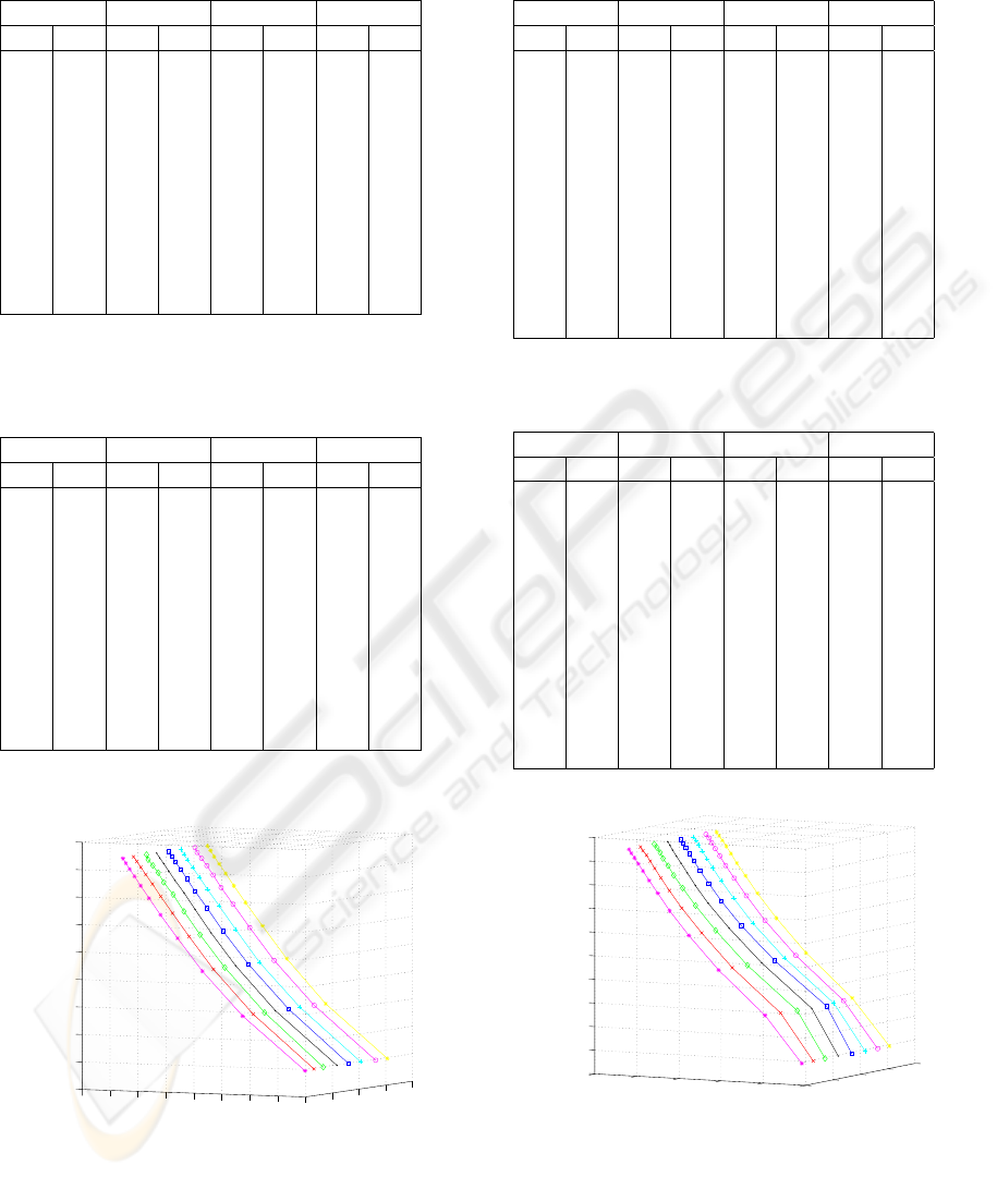
Table 2: Low sensor calibration data. The four first LED
bars Bi
L
.
B1
L
B2
L
B3
L
B4
L
radius α radius α radius α radius α
370.96 33.17 371.74 78.28 366.44 122.80 366.28 168.66
260.94 33.49 261.46 77.23 257.22 122.88 259.10 168.87
191.43 33.62 190.12 78.03 185.00 123.09 186.96 168.89
147.67 32.80 145.78 76.92 142.21 122.45 141.79 168.61
116.81 32.05 115.54 75.77 113.42 123.11 113.09 168.78
96.39 32.64 94.50 76.77 92.56 123.71 91.88 169.33
81.03 31.21 79.67 75.11 77.42 122.91 77.02 168.77
69.95 31.93 67.65 73.89 66.17 123.79 66.28 168.69
60.68 31.82 58.95 75.21 57.65 125.39 57.02 169.90
53.67 30.19 51.53 75.96 50.93 124.45 50.10 169.65
47.90 30.06 46.02 72.93 44.91 122.20 44.66 168.37
Table 3: Low sensor calibration data. The four last LED
bars Bi
L
.
B5
L
B6
L
B7
L
B8
L
radius α radius α radius α radius α
367.38 213.91 364.42 259.22 369.42 304.89 375.05 349.70
256.71 213.58 259.43 259.38 261.23 305.37 263.51 349.94
186.34 214.66 188.20 259.40 189.89 305.28 191.15 349.75
142.42 214.66 144.23 259.90 145.87 304.65 146.91 349.80
113.46 213.72 115.05 259.15 116.19 304.28 116.27 349.59
93.64 213.73 95.13 257.85 95.60 305.32 95.84 349.78
77.43 213.73 79.17 260.10 80.81 305.24 81.01 350.04
66.20 213.97 67.86 256.52 69.36 306.15 70.11 350.14
57.87 214.76 59.16 258.62 60.21 305.53 61.04 349.61
50.59 214.96 51.70 260.53 53.63 306.70 54.22 349.37
45.26 215.05 46.42 255.76 47.74 307.26 49.07 349.43
0
50
100
150
200
250
300
350
400
0
100
200
300
400
−10
0
10
20
30
40
50
60
70
80
alpha
radius
gamma
Figure 8: Illustration of the function γ = f (α, r) obtained
for the low sensor.
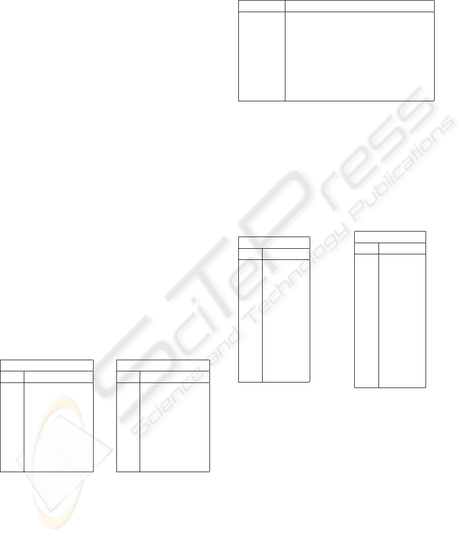
Table 4: High sensor calibration data. The four first LED
bars Bi
H
.
B1
H
B2
H
B3
H
B4
H
radius α radius α radius α radius α
460.37 32.89 461.61 77.69 461.45 122.77 458.85 167.92
371.57 32.38 380.46 77.19 386.66 121.97 398.91 167.84
262.05 32.29 267.33 77.50 269.95 122.76 275.66 167.64
192.46 33.06 194.41 77.76 194.35 122.45 196.32 167.34
146.95 32.51 148.70 75.55 148.37 121.13 148.38 167.15
119.07 33.08 119.80 75.51 119.17 122.06 118.37 166.81
98.84 33.80 99.83 76.31 99.08 122.02 97.36 166.33
84.30 33.06 85.68 75.61 84.65 121.73 82.62 165.99
72.93 32.32 74.46 75.21 73.25 120.67 71.55 166.25
64.08 33.10 65.42 74.36 64.86 120.30 63.06 165.30
56.91 34.21 58.49 73.21 58.00 120.45 56.14 165.56
51.83 35.36 52.66 75.56 52.04 122.27 50.68 165.13
Table 5: High sensor calibration data. The four last LED
bars Bi
H
.
B5
H
B6
H
B7
H
B8
H
radius α radius α radius α radius α
456.26 213.07 454.36 258.34 454.99 302.67 457.48 348.01
393.00 212.64 388.01 257.62 376.95 301.90 370.19 348.15
273.74 211.98 268.91 256.98 262.48 302.24 260.10 348.01
196.09 211.68 193.45 256.36 190.56 302.90 189.86 348.76
145.99 211.37 145.36 255.92 143.81 303.44 144.52 349.23
115.96 211.15 114.59 255.60 114.39 303.85 116.84 349.64
96.13 210.64 94.34 257.20 94.82 304.65 96.37 349.84
81.24 210.30 79.66 255.13 80.15 304.56 81.93 350.16
70.22 210.83 68.82 256.76 69.17 304.51 71.24 351.11
61.22 210.41 60.26 254.22 60.71 304.56 62.18 350.74
54.49 209.69 53.03 254.05 53.45 306.43 55.35 351.69
49.05 209.29 47.41 255.98 47.88 307.48 49.81 351.92
0
100
200
300
400
500
0
100
200
300
400
−20
−10
0
10
20
30
40
50
60
70
80
alpha
radius
gamma
Figure 9: Illustration of the function γ = f (α, r) obtained
for the high sensor.
VISAPP 2006 - IMAGE FORMATION AND PROCESSING
16
6 DISCUSSION
From the results presented, two main points can be
discussed.
The markers positioned onto a same vertical bar must
have, theoretically, similar angle α values either for
the low sensor or the high sensor. Considering the
low sensor, the mean deviation fluctuates from 0.183
to 1.306 (cf. Table 6) (all the quantities enumerated
in this paragraph are in pixel unity). In the case of
the high sensor, the mean deviation varies from 0.643
to 1.137 (cf. Table 7). The difference of the mean
α values of the low and high sensors gives informa-
tion about the alignment of the sensors on a com-
mon optical axis. This difference varies from 0.029
to 3.119 (cf. Table 8). The vertical alignment of the
sensors is one of the main requirement for the devel-
opment of stereovision sensors. This parameter has
an effect on two notions. The first one deals with the
self-calibration and more precisely the establishment
of the fundamental and essential matrices. Thus, a
too important error may affect significantly the pixel
matchings. The second one is linked to the resolu-
tion of the sensor. A misalignment of the two sensors
implying an error of 3.119 may be sufficient for ap-
plications which do not require a high resolution, and
probably not for fine applications.
From the different experiences conducted, it is dif-
ficult to realize a perfect alignment in hardware imple-
mentation. An alignment correction by an analytical
procedure is envisaged to break of this problem.
Table 6: Mean deviation of
the parameter α in the case
of the low sensor.
Low Sensor
Mean deviation of α
B1
L
0.959
B2
L
1.306
B3
L
0.720
B4
L
0.366
B5
L
0.520
B6
L
1.148
B7
L
0.651
B8
L
0.183
Table 7: Mean deviation of
the parameter α in the case
of the high sensor.
High Sensor
Mean deviation of α
B1
H
0.643
B2
H
1.112
B3
H
0.718
B4
H
0.845
B5
H
0.894
B6
H
1.043
B7
H
1.267
B8
H
1.137
A similar analysis can be developed in the case of
the radius parameter r. The markers located at a same
altitude must have, theoretically, equal radius values.
For the low sensor the mean deviation fluctuates from
1.201 to 2.833 (cf. Table 9). In the case of the high
sensor this deviation fluctuates from 1.590 to 2.399
(cf. Table 10). The value 8.427 is not taken into ac-
count because it is not a relevant value towards the
homogeneousness of the values obtained. This eval-
uation is linked to the alignment between the verti-
Table 8: Evaluation of the difference of the mean values α.
Highlighting of the difficulty to get a common optical axis
for the two sensors.
Difference of the mean value of the parameter α
B1
L
/B1
H
1.083
B2
L
/B2
H
0.055
B3
L
/B3
H
1.629
B4
L
/B4
H
2.351
B5
L
/B5
H
3.119
B6
L
/B6
H
2.587
B7
L
/B7
H
1.417
B8
L
/B8
H
0.029
cal axis of the frame of the test-pattern (Z
TP
) and
the optical axis of the panoramic stereovision sensor.
In hardware implementation, it is difficult to merge
the two axes. An analytical procedure is envisaged to
break of this problem.
Table 9: Mean deviation of
the parameter r in the case
of the low sensor.
Low Sensor
Mean radius
h
1
2.833
h
2
1.834
h
3
2.009
h
4
1.948
h
5
1.240
h
6
1.312
h
7
1.434
h
8
1.392
h
9
1.201
h
10
1.345
h
11
1.434
Table 10: Mean deviation
of the parameter r in the
case of the high sensor.
High Sensor
Mean radius
h
3
2.399
h
4
8.427
h
5
4.537
h
6
1.858
h
7
1.590
h
8
1.830
h
9
1.682
h
10
1.786
h
11
1.590
h
12
1.628
h
13
1.652
h
14
1.631
7 CONCLUSION
The main objective of this article is to present an
innovative calibration method applied to a panoramic
stereovision sensor. The sensor presented is made of
two catadioptric sensors coupled vertically with their
optical axis in common. The calibration technique is
based on the characteristics of the images obtained
by a catadioptric sensor. A pixel or sub-pixel can
be expressed in polar coordinates (α, r) and the
radius r is linked to the coordinates of the point
expressed in the 3D frame. Thus, we use a low-cost
cylindrical test-pattern made of several markers
which cylindrical coordinates are known. Classical
image algorithms are applied to determine the polar
AN EFFICIENT CATADIOPTRIC SENSOR CALIBRATION BASED ON A LOW-COST TEST-PATTERN
17

coordinates of the pixel or sub-pixel matching. The
function linking the 3D points to the 2D points is
obtained and a local bilinear interpolation is carried
out to get the 3D/2D matchings for points which 3D
coordinates are known.
Three main perspectives of work are envisaged.
• The first one consists in developing analytical pro-
cedures which enable the correction of the mis-
alignment of the two sensors and the misalignment
between the optical axis and the vertical axis of the
frame of the test-pattern.
• The second one is linked to the development of an
analytical calibration method which is based on the
minimization of a criterion function. This function
is defined as the non-linear equation linking a 3D
point considered in the environment and a 2D point
on the image plane (Svoboda, 1999). We propose
to use the Levenberg-Marquardt algorithm which
is a classical optimization technique for non-linear
equation.
• The third one deals with the self-calibration of the
panoramic stereovision sensor. It consists in the es-
tablishment of the fundamental and essential matri-
ces. This calibration method is linked to the epipo-
lar geometry which enables the matchings of pixels
in different image planes. This geometry is well
known for classical vision systems and has been
recently established for catadioptric sensors (Svo-
boda, 1999).
REFERENCES
Aliaga, D. (2001). Accurate catadioptric calibration for
real-time pose estimation inroom-size environments.
In 8th IEEE International Conference on Computer
Vision, volume 1, pages 127–134.
C. Cauchois, E. Brassart, C. P. and Clerentin, A. (1999).
Technique for calibrating an omnidirectional sensor.
In International Conference on Intelligent Robots and
Systems.
C. Drocourt, L. Delahoche, E. B. and Cauchois, C. (2001).
Simultaneous localization and map building paradigm
based on omnidirectional stereoscopic vision. In Pro-
ceeding IEEE Workshop on Omnidirectional Vision
Applied to Robotic Orientation and Nondestructive
Testing, pages 73–79.
C. Geyer, K. D. (2001). Catadioptric projective geometry.
International Journal of Computer Vision, 43:223–
243.
F. Marzani, Y. Voisin, A. D. and Voon, L. F. L. Y. (2002).
Calibration of a 3d reconstruction system using a
structured light source. Journal of Optical Engineer-
ing, 41:484–492.
Faugeras, O. (1993). Three-dimensional computer vision
: a geometric viewpoint. MIT Press, Cambridge,
Massachusetts, 4th edition.
G.L. Mariottini, D. P. (2005). The epipolar geometry tool-
box : multiple view geometry for visual servoing for
matlab. IEEE Robotics and Automation Magazine.
J. Fabrizio, J.-P. Tarel, R. B. (2002). Calibration of
panoramic catadioptric sensors made easier. In Work-
shop on Omnidirectional Vision.
J.P. Barreto, H. A. (2005). Geometric properties of central
catadioptric line images and their application in cali-
bration. IEEE Transactions on Pattern Analysis and
Machine Intelligence, 27:1327–1333.
Kang, S. (2000). Catadioptric self-calibration. In Inter-
national Conference on Computer Vision and Pattern
Recognition, volume 1, pages 201–207.
L. Smadja, R. Benosman, J. D. (2004). Cylindrical sensor
calibration using lines. In 5th Workshop on Omnidi-
rectional Vision, Camera Networks and Non-Classical
Cameras, pages 139–150.
Lacroix, S., Gonzalez, J., El Mouaddib, M., Vasseur, P.,
Labbani, O., Benosman, R., Devars, J., and Fabrizio,
J. (2005). Vision omnidirectionnelle et robotique. rap-
port final. Technical report, LAAS, CREA, LISIF.
Moldovan, D. (2004). A geometrically calibrated pinhole
model for single viewpoint omnidirectional imaging
systems. In British Machine Vision Conference.
Mouaddib, M. E. (2005). La vision omnidirectionnelle. In
Journée Nationale de la Recherche en Robotique.
P. Biber, H. Andreasson, T. D. and Andreas, A. S. (2004).
3d modeling of indoor environments by a mobile ro-
bot with a laser scanner and panoramic camera. In
IEEE/RSJ International Conference on Intelligent Ro-
bots and Systems.
S. Baker, S. N. (1999). A theory of single-viewpoint cata-
dioptric image formation. International Journal of
Computer Vision, 35:175–196.
S. Baker, S. N. (2001). Panoramic Vision: Sensors, The-
ory and Applications, chapter Single viewpoint cata-
dioptric cameras, pages 39–73. Springer-Verlag, 1st
edition.
Svoboda, T. (1999). Central panoramic cameras. Design,
geometry, egomotion. PhD thesis, Czech Technical
Univeristy.
T. Ea, O. Romain, C. G. and Garda, P. (2001). Un capteur
de sphéréo-vision stéréoscopique couleur. In Congrès
francophone de vision par ordinateur ORASIS.
T. Svoboda, T. Pajdla, V. H. (1998). Epipolar geometry for
panoramic cameras. In 5th European Conference on
Computer Vision, volume 1406, pages 218–232.
X. Ying, Z. H. (2003). Catadioptric camera calibration us-
ing geometric invariants. In International Conference
on Computer Vision, pages 1351–1358.
Zhu, Z. (2001). Omnidirectional stereo vision. In 10th IEEE
ICAR Workshop on Omnidirectional Vision.
VISAPP 2006 - IMAGE FORMATION AND PROCESSING
18
