
RESTORATION OF DEGRADED MOVING IMAGE FOR
PREDICTING A MOVING OBJECT
Kei Akiyama
1),2)
, Zhi-wei Luo
2)
, Masaki Onishi
2)
and Shigeyuki Hosoe
1),2)
1) Graduate School of Engineering, Nagoya University
Furo-cho, Chikusa-ku Nagoya, 464-8603 JAPAN
2)
Bio-mimetic Control Research Center, RIKEN
2271-130, Anagahora, Shimoshidami, Moriyama-ku Nagoya, 463-0003 JAPAN
Keywords:
Moving image restoration, wavelet multiresolution analysis, nonlinear optimization, dynamics of moving im-
age.
Abstract:
Iterative optimal calculation methods have been proposed for restoration of degraded static image based on
wavelet multiresolution decomposition. However, it is quite difficult to apply these methods to process mov-
ing images due to the high computation cost. In this paper, we propose an effective restoration method for
degraded moving image by modeling the motion of a moving object and predicting the future object position.
We verified our method by computer simulations and an experiment to show that our method can reduce the
computation time.
1 INTRODUCTION
When measuring external world by a camera, degra-
dation in the observed images may be caused by many
factors. It is then important to estimate the original
image and to restore the observed one. By now, in the
research field of computer vision, there are several ap-
proaches be proposed for degraded image restoration
(Geman and Yang, 1995; Osher et al., 1992; Belge
et al., 2000). One of these approaches (Belge et al.,
2000) even enables the edge-preserving restoration of
an image by using wavelet multiresolution decom-
position (Mallat, 1989). However, because of huge
amount of computation cost, this approach can only
be applied for the restoration of a static image but is
ineffective to process the moving image.
In this paper, we propose a novel restoration
method for a moving image by developing the Belge
et al.’s approach. In our algorithm, we model the dy-
namics of moving image and calculate the restored
image using the predicted image that is calculated
based on the dynamic model of the moving object.
We verify our method by computer simulation of arti-
ficially generated moving image and an experiment of
a real moving image, which show that our method can
realize image restoration while reducing computation
time.
2 STATIC IMAGE RESTORATION
In this section, we first review the restoration method
for a static image (Belge et al., 2000) using wavelet
multiresolution decomposition.
A general degradation process of an N × N static
image can be formulated as
g = Hf + u (1)
where the vectors g, f and u represent the lexico-
graphically ordered degraded image, the original im-
age and the disturbance, respectively. The matrix H
represents optical blur or linear distortion. With 2-D
wavelet multiresolution (Mallat, 1989), equation (1)
can be converted into the following form
ˆ
g =
ˆ
H
ˆ
f +
ˆ
u (2)
where
ˆ
g,
ˆ
H,
ˆ
f,
ˆ
u are
ˆ
g = Wg,
ˆ
f = Wf ,
ˆ
u = Wu
and
ˆ
H = WHW
T
with a wavelet multiresolution
decomposition matrix W, respectively. W is orthog-
onal, that is W
T
W = I.
Wavelet multiresolution decomposition is a method
of decomposing an image into multiresolution im-
ages by utilizing orthogonal wavelet transformation.
A block diagram of two level wavelet decomposition
of image f is shown in Fig. 1, in which p(·) and q(·)
are 1-D low-pass and high-pass filters. From the input
image, four down-sampled images (LL, HL, LH, HH)
72
Akiyama K., Luo Z., Onishi M. and Hosoe S. (2006).
RESTORATION OF DEGRADED MOVING IMAGE FOR PREDICTING A MOVING OBJECT.
In Proceedings of the First International Conference on Computer Vision Theory and Applications, pages 72-79
DOI: 10.5220/0001373700720079
Copyright
c
SciTePress

(HL)
(LH)
(HH)
p(n)
p(n)
2
q(n)
q(n)
2
2
2
2
f
(1,1)
^
f
(1,2)
^
f
(1,3)
^
p(m)
q(m)
f
2
Input image
(LL)
f
(2,0)
^
Level 2
(HL)
(LH)
(HH)
p(n)
p(n)
2
q(n)
q(n)
2
2
2
2
f
(2,1)
^
f
(2,2)
^
f
(2,3)
^
p(m)
q(m)
2
(LL)
f
(1,0)
^
Level 1
p( ), q( ) : 1-D Filter
2
: Downsampling
n : Vertical direction
m : Horizontal direction
.
.
Figure 1: Two level multiresolution wavelet decomposition
of an image f .
are obtained. Furthermore, by repeating the decom-
position, we can get multiresolution images. Note that
the number of the total pixels is unchanged during the
decomposition.
The optimal restored image for the degradation
process (2) is obtained by minimizing the next cost
function about
ˆ
f (Belge et al., 2000)
J
ˆ
f, λ
=
ˆ
g −
ˆ
H
ˆ
f
2
2
+ λ
(L,0)
ˆ
f
(L,0)
p
p
+
L
l=1
3
j=1
λ
(l,j)
ˆ
f
(l,j)
p
p
.
(3)
The subscript l and j denote the decomposition level
and the type of the decomposed image, respectively.
The optimal restored image can be obtained by cal-
culating
ˆ
f
∗
such that the differentiation of the cost
function (3) approaches to 0. Then we get
ˆ
H
T
ˆ
H +
p
2
D
∗
ˆ
f
∗
=
ˆ
H
T
ˆ
g (4)
D
∗
= diag
λ(i)
(|
ˆ
f
∗
(i)|
2
+ β)
1−p/2
N
2
i=1
(5)
(Belge et al., 2000). Here,
ˆ
f
∗
(i) denotes the ith ele-
ment of
ˆ
f
∗
, λ(i) is the weight corresponds to
ˆ
f
∗
(i),
and β(≥ 0) is the stabilization constant for approxi-
mation of L
p
norm terms (Belge et al., 2000), respec-
tively.
To solve this nonlinear equation, an iterative calcu-
lation method can be applied as follows (Belge et al.,
2000)
ˆ
H
T
ˆ
H +
p
2
D
(k)
ˆ
f
(k+1)
=
ˆ
H
T
ˆ
g (6)
D
(k)
= diag
λ(i)
(|
ˆ
f
(k)
(i)|
2
+ β)
1−p/2
N
2
i=1
(7)
where the superscript (k) expresses an iteration num-
ber of times. If p ≥ 1 and
ˆ
H is full rank, it is shown
that the iterative calculation by (6) and (7) converges
to the solution of the nonlinear equations (4) and (5)
(
ˆ
f
∗
) with a suitable initial value
ˆ
f
(0)
when k →∞
(Charbonnier et al., 1997).
The above method can remove the degradation fac-
tors while preserving local patterns of an image by
assigning different weight λ
(l,j)
to each decomposed
image. Here, λ is set as a constant for simplicity.
3 MOVING IMAGE
RESTORATION
3.1 Application to the Moving Image
Restoration
In this paper, we consider the moving image restora-
tion problem to restore a time series of original im-
ages (f
[1]
, ··· , f
[K]
) from a degraded time series of
observed images (g
[1]
, ··· , g
[K]
). Here, it is noted
that the superscript [k] expresses a frame number of a
moving image whereas the superscript (k) in equa-
tions (6) and (7) expressed the iteration number of
times.
We suppose that a degradation process of an image
is similar to the case of static image:
g
[k]
= Hf
[k]
+ u
[k]
,k=1, ··· ,K. (8)
In this work, we assume H to be constant, that is, the
optical blur or the distortion is independent of each
frame.
Since equations (6) and (7) represent iterative cal-
culation with a huge (order(N
2
)) matrix, it requires
high computational cost when applying this algorithm
directly in our moving image restoration. Therefore,
we assume the following properties about the original
moving image and propose our approach to reduce the
calculation cost.
Assumption about an original image
1. An original moving image consists of a foreground
and a background.
2. The change of the background is so small so as be
set as a static image.
3. The change of the foreground can be formulated or
be approximated by known dynamics such as linear
or parabolic movements as will be mentioned later.
4. The foreground is assumed to be a single rigid body
with smoothly changing pixel value in the domain
and maintain its orientation.
When the assumptions 1 and 2 hold, we can utilize the
restoration result of previous frame directly as an ini-
tial estimation of the background for each frame. On
the other hand, we can predict a new position of the
foreground from the previous restoration result and
the information about motion dynamics (assumption
RESTORATION OF DEGRADED MOVING IMAGE FOR PREDICTING A MOVING OBJECT
73

Degraded
Images
Restored
Images
Calculation of Predicted Image
g
f
rest
f
mask
v
f
pred
f
f
mask
, f
fg
g
f
rest
, f
fg
pred
[k]
[k]
[k]
~
~
Moving object estimation
Prediction of feature point velocity
Moving object prediction
Predicted image calculation
f
rest
f
rest
f
rest
Restoration
(eq. 9 and 10)
g
[k]
g
[k-1]
g
[k-2]
k
k
[k]
[k]
[k]
[k-1]
[k-1]
[k][k]
[k-1]
[k]
[k-1]
[k-2]
T
Figure 2: Overview of the proposed method at kth frame.
3) by using Kalman filter. Therefore, by using these
images as an initial value in the equations (6) and (7),
we can show that good restoration results can be ob-
tained by only one time restoration calculation, in sec-
tion 4. In addition, for the moving image which stood
static, our algorithm agrees with the Belge et al.’s al-
gorithm.
Based on the above description, we modify the
foregoing iterative calculation (6) and (7) as follows:
ˆ
H
T
ˆ
H +
p
2
D
[k]
pred
ˆ
f
[k]
rest
=
ˆ
H
T
ˆ
g
[k]
(9)
D
[k]
pred
= diag
λ(i)
(|
ˆ
f
[k]
pred
(i)|
2
+ β)
1−p/2
N
2
i=1
. (10)
Here,
ˆ
f
[k]
rest
is a restored image of kth frame in the
wavelet domain, and
ˆ
f
[k]
pred
is a predicted image of kth
frame. We denote a restored and a predicted images in
space domain as f
[k]
rest
and f
[k]
pred
. A summary of our
proposed method is shown in Fig. 2. The dynamics
of the moving image will be formulated later and will
be used to calculate the predicted image
ˆ
f
[k]
pred
.For
a degraded image
ˆ
g
[k]
, we calculate a restored image
f
[k]
rest
by equations (9) and (10) using
ˆ
f
[k]
pred
.
3.2 Formulation Dynamics of
Moving Image
Based on the above assumptions, we model dynamics
of an original moving image as follows. At first we
define each variables.
f
[k]
FOriginal image vector of kth frame
f
[k]
mask
FOriginal moving object domain vector
f
bg
FOriginal background image vector
f
[k]
fg
FOriginal foreground image vector
Original moving object domain vector is a vector in
which pixels where the background is covered behind
the moving object are 0, and the others are 1. Original
foreground image vector is made by turned over with
0 and 1 of f
[k]
mask
, and multiplied by the original pixel
value of the moving object. All the vectors are with
N
2
dimension. By the definitions, they satisfy
f
[k]
= diag
f
bg
(1),...,f
bg
(N
2
)
· f
[k]
mask
+ f
[k]
fg
.
(11)
For transition of moving object domain f
[k]
mask
with
constant acceleration for an example, we get
f
[k+1]
mask
= T
v
[k]
f
[k]
mask
(12)
v
[k+1]
a
[k+1]
=
II
0 I
v
[k]
a
[k]
. (13)
We call T (v
[k]
) a transition matrix. Vectors v
[k]
=
(v
[k]
x
,v
[k]
y
)
T
and a
[k]
=(a
[k]
x
,a
[k]
y
)
T
are velocity and
acceleration of the moving object, and subscripts x, y
express vertical and horizontal directions. From the
assumption 4, we can regard transition of an moving
object as a translation. Therefore, transition matrix
can be expressed as follows:
T
v
[k]
= diag
C
y
v
[k]
y
,...,C
y
v
[k]
y
· C
x
v
[k]
x
.
(14)
Matrix C
x
and C
y
in equation (14) are following
N
2
×N
2
dimension block circulant matrix and N ×N
dimension circulant matrix:
C
x
=
⎡
⎢
⎢
⎢
⎢
⎢
⎢
⎣
00 0··· 0 I
I 00··· 00
0 I 0 ··· 00
.
.
.
.
.
.
.
.
.
.
.
.
.
.
.
.
.
.
0 ··· 0 I 00
0 ··· 00I 0
⎤
⎥
⎥
⎥
⎥
⎥
⎥
⎦
(15)
C
y
=
⎡
⎢
⎢
⎢
⎢
⎢
⎢
⎣
00 0··· 01
10 0··· 00
01 0··· 00
.
.
.
.
.
.
.
.
.
.
.
.
.
.
.
.
.
.
0 ··· 0100
0 ··· 0010
⎤
⎥
⎥
⎥
⎥
⎥
⎥
⎦
. (16)
Here, we express them with
C
−v
[k]
x
x
:=
C
x
−1
v
[k]
x
, C
−v
[k]
y
y
:=
C
y
−1
v
[k]
y
in the case of v
[k]
x
= −v
[k]
x
< 0 or v
[k]
y
= −v
[k]
y
< 0.
In addition, the transition of foreground image f
[k+1]
fg
is provided by the same transition matrix T (v
[k]
).
Moreover, we can describe the rotation or the ex-
pansion / reduction of an moving object domain by
modeling the transition matrix.
3.3 Algorithm for Moving Image
Restoration
The moving image restoration algorithm is given as
follows:
VISAPP 2006 - IMAGE FORMATION AND PROCESSING
74

Moving image restoration algorithm in K
frames
1. Give a predicted image
ˆ
f
[1]
pred
when k =1, prop-
erly.
2. Calculate the restored image
ˆ
f
[k]
rest
by equations (9)
and (10) with
ˆ
f
[k]
pred
for the degraded image
ˆ
g
[k]
.
Calculate f
[k]
rest
= W
T
ˆ
f
[k]
rest
.
3. Calculate an estimation of a moving object domain
(
˜
f
[k]
mask
) from f
[k]
rest
.
4. With
˜
f
[k]
mask
, divide f
[k]
rest
into the estimated fore-
ground (
˜
f
[k]
fg
) and background (
˜
f
[k]
bg
). For each
pixel, if
˜
f
[k]
mask
[(n − 1)N + m]=1, then
˜
f
[k]
fg
[(n − 1)N + m]:=0, and
˜
f
[k]
bg
[(n − 1)N + m]:=f
[k]
rest
[(n − 1)N + m].
Else, if
˜
f
[k]
mask
[(n − 1)N + m]=0, then
˜
f
[k]
fg
[(n − 1)N + m]:=f
[k]
rest
[(n − 1)N + m], and
˜
f
[k]
bg
[(n − 1)N + m]:=0,
(n =1, ··· ,N, m =1, ··· ,N).
5. Detect a certain characteristic point c
[k]
=
(c
[k]
x
,c
[k]
y
)
T
(center of gravity, for example) of
˜
f
[k]
fg
,
and calculate a predicted value (
¯
c
[k+1]
)ink +1th
frame by Kalman filter. Calculate a predicted ve-
locity (
¯
v
[k]
) and the transition matrix T (
¯
v
[k]
) suc-
cessively. Calculate a predicted moving object do-
main (
¯
f
[k+1]
mask
) by:
¯
f
[k+1]
mask
:= T (
¯
v
[k]
)
˜
f
[k]
mask
. (17)
6. Calculate the predicted foreground image (
¯
f
[k+1]
fg
)
using the transition matrix T (
¯
v
[k]
) and
˜
f
[k]
fg
. Cal-
culate the predicted background image (
¯
f
[k+1]
bg
)by
taking average of
˜
f
[l]
bg
(l =1, ··· ,k) for each pixel.
7. With
¯
f
[k+1]
mask
,
¯
f
[k+1]
fg
and
¯
f
[k+1]
bg
provided by steps 5
and 6, calculate the predicted image f
[k+1]
pred
by the
next expression corresponding to equation (11).
f
[k+1]
pred
:= diag
¯
f
[k+1]
bg
(1),...,
¯
f
[k+1]
bg
(N
2
)
·
¯
f
[k+1]
mask
+
¯
f
[k+1]
fg
(18)
Calculate
ˆ
f
[k+1]
pred
= Wf
[k+1]
pred
.
8. Repeat the steps 2 to 7 for k =1, ··· ,K. Termi-
nate at step 2 for k = K.
In addition, if we could not predict it for the reasons
of frame-out of the moving object or an change of the
Table 1: Parameters used in the simulation.
item name value
Optical blur (σ
2
) 1.7
SN ratio of the disturbance
15dB
Level of the decomposition(L) 3
(λ
1
, λ
2
) (0.1, 0.3)
p
1.0
α
1.2
β
10
−2
scene, we cancel the prediction till the next moving
object is observed.
Considering the limited paper length we eliminated
the detailed calculations in steps 3 and 5.
4 SIMULATION STUDIES
We performed a simulation of the proposed method
for an artificially generated and a real moving im-
ages. The artificial moving image has known degra-
dation parameters and we verified the performance of
the proposed method quantitatively. The degradation
parameters of the real moving image are unknown, so
we verified it qualitatively.
4.1 Restoration Simulation of an
Artificial Moving Image
We generated an artificial moving image in 128×128
pixels and 36 frames. We used a test image LAX for
the background and an arbitrary-shaped object with
uniform pixel value for the foreground. The fore-
ground was supposed to move with constant velocity.
We made the original moving image f
[k]
by equation
(11) and calculated its degraded moving image g
[k]
by equation (8). In addition, we considered an optical
blur for H in equation (8) and used a Gauss function
of the variance σ
2
=1.7 with the 9 × 9 discretized
elements. In addition, the disturbance u
[k]
was as-
sumed to be a Gaussian noise of average of 0 and SN
ratio of 15dB independent between each frames. In
the restoration calculation, the level of the wavelet
multiresolution decomposition (L) was assumed to
be 3 and used the three tap wavelet (Daubechies,
1992). Besides, the parameter λ
(l,j)
was set as fol-
lows (Belge et al., 2000):
λ
(3,0)
= λ
1
,λ
(l,j)
= λ
2
2
−α(l−3)
(l =1, 2,j=1, 2, 3)
(19)
The parameters we used in the simulation are given
in Table 1. The predicted image in step 1 of the
proposed algorithm was assumed to be
ˆ
f
[1]
pred
=
ˆ
g
[1]
.
In addition, we did not calculate predicted images and
RESTORATION OF DEGRADED MOVING IMAGE FOR PREDICTING A MOVING OBJECT
75
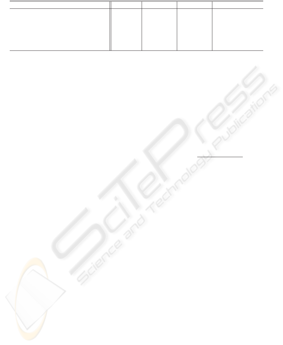
Table 2: Comparison of the simulation result of 32nd frame.
item name Proposed Compared 1 Compared 2 (Belge et al., 2000)
Cost value of a restored image (×10
5
) 1.54 1.52 1.52 1.50
Cost value of an initial image (×10
5
) 1.85 5.15 3.96 3.96
ISNR[dB]
3.27 3.25 3.14 2.54
Iterative calculation number of times
1 2 2 30
Calculation time
2’38” 5’20” 5’00” 1:14’17”
Prediction time (of which calc. time)
1” — — —
just set
ˆ
f
[k+1]
pred
:=
ˆ
f
[k]
rest
in k =1, 2 and 3 because
there existed a big change in the restored images of
these frames. We calculated the predicted images in
the other frames.
We compared our approach with the following two
cases.
• With the restored image of previous frame for the
initial value, iterate calculation of equations (6) and
(7) till the cost value of a restored image in the pro-
posed method is provided in each frame (compared
method 1).
• With the current degraded image for the initial
value, iterate calculation of equations (6) and (7)
till the cost value of a restored image in the pro-
posed method is provided in each frame (compared
method 2).
4.1.1 Simulation Result for One Representative
Frame
We compare a restoration result of 32nd frame as an
example here. We show numerical values of the re-
stored images of each method in Table 2. Moreover,
for reference, we also show numerical values of a
restoration result of the method in which
• With the current degraded image for the initial
value, iterate calculation of equations (6) and (7)
till it converges in each frame (Belge et al.’s
method)
in the table. Here, we judged the restored image
of k
th iteration number of times of 32nd frame
(
ˆ
f
[32](k
)
rest
) to have converged when
ˆ
f
[32](k
)
rest
−
ˆ
f
[32](k
−1)
rest
ˆ
f
[32](k
−1)
rest
< 5.0×10
−4
and broke off the calculation (Belge et al., 2000).
In the first and second lines of the table, we show
the cost values which were calculated for a restored
image or an initial image by the following cost func-
tion
J
ˆ
η
[k]
, λ
=
ˆ
g
[k]
−
ˆ
H
ˆ
η
[k]
2
2
+ λ
(L,0)
ˆ
η
[k]
(L,0)
p
p
+
L
l=1
3
j=1
λ
(l,j)
ˆ
η
[k]
(l,j)
p
p
(20)
corresponding to equation (3). In the second line,
an initial image of each method corresponds to the
predicted image (proposed method), the restored im-
age of previous frame (compared method 1) and the
current degraded image (compared method 2 and the
Belge et al.’s method). The cost value of the predicted
image of the proposed method is smaller than those of
the initial images of the compared method 1 and 2.
In the third line, we show ISNR (Improved Signal
to Noise Ratio) (Banham and Katsaggelos, 1997) cal-
culated by the next equation:
ISNR = 10 log
10
g
[k]
− f
[k]
2
f
[k]
rest
− f
[k]
2
[dB] . (21)
ISNR of the proposed method is 3.27dB, which is an
enough good restoration result. In addition, ISNR of
the proposed method is similar as a result of the com-
pared method 1, and be better than that of the com-
pared method 2. On the other hand, ISNR of the
Belge et al.’s method is smaller, however, it is good
from the subjective evaluation as will be mentioned
later. Such a tendency can be seen in other frames.
Furthermore, we show the iterative calculation
number of times of each method in the fourth line. In
the fifth line, we show the each calculation time. The
prediction time in our proposed method is shown in
sixth line. Since we did not predict it except the pro-
posed method, we denote them by —. As for the pro-
posed method, a restored image is provided by only
one calculation whereas more than two times calcu-
lation were needed for the other methods. Accord-
ingly, the calculation time of the compared methods
were around twice the length of that of our proposing
method. Note that 30 times of iteration were neces-
sary for the Belge’s method and the calculation time
was more than one hour. In contrast, the prediction
time of our method is extremely short.
We compare the restored images of each method
next. We show the original image f
[32]
in Fig. 3. A
certain gray domain in the vicinity of the center of
the image is a moving object. We show the degraded
image g
[32]
in Fig. 4. From the degraded image, dis-
tinction of the detail patterns in the original image is
difficult.
VISAPP 2006 - IMAGE FORMATION AND PROCESSING
76
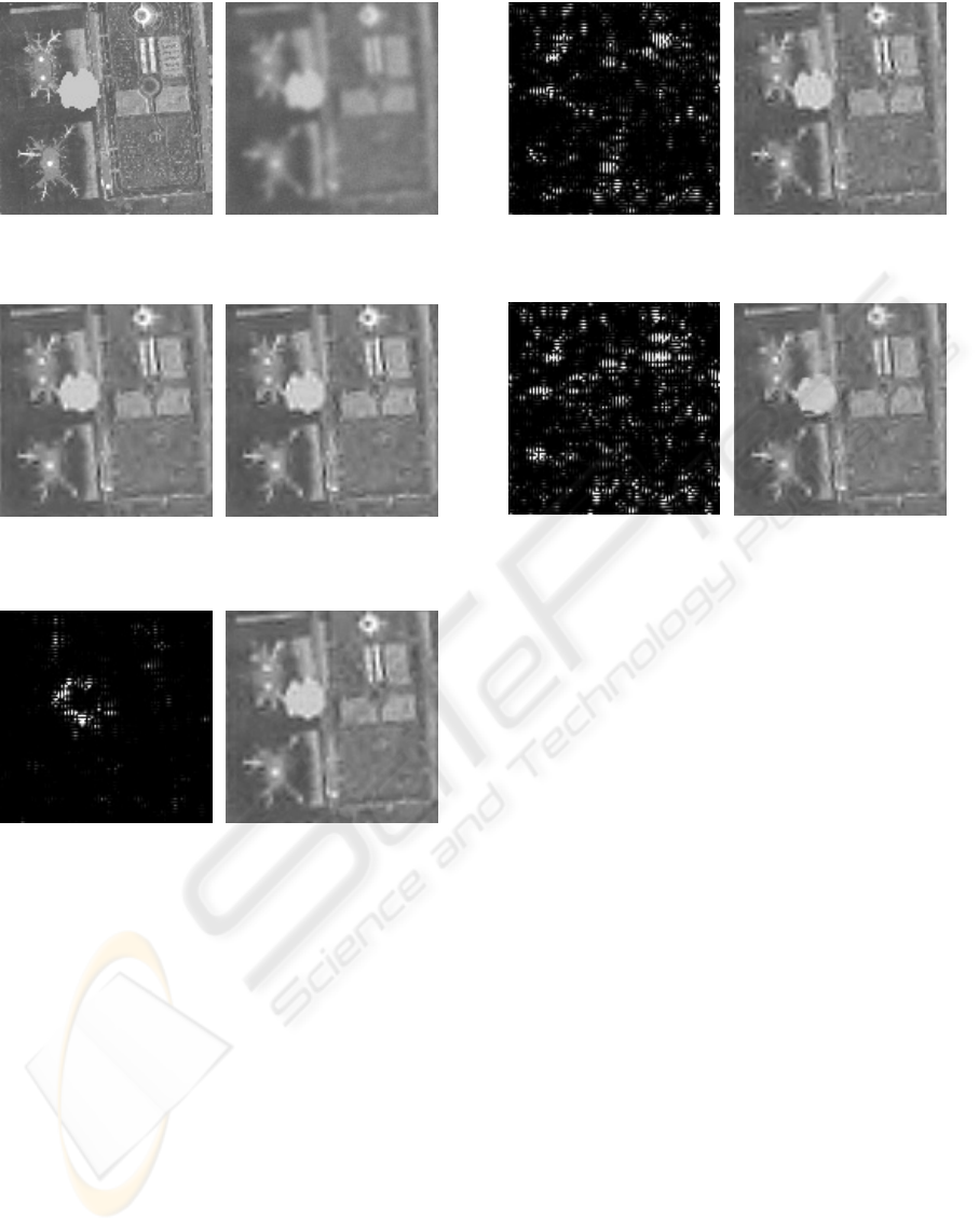
Figure 3: Original image
(f
[32]
).
Figure 4: Degraded image
(g
[32]
).
Figure 5: Restored image
(proposed method).
Figure 6: Restored image
(compared method 1).
Figure 7: Squared error
of Fig. 5 and Fig. 6.
Figure 8: Restored image
(compared method 2).
We show the restored image f
[32]
rest
by our method
in Fig. 5. We can see that the edge in Fig. 5 is clearer
than those in Fig. 4, and detailed patterns in Fig. 3
appear in the restored image to some extent. On the
other hand, we show the restored image of the com-
pared method 1 in Fig. 6. Comparing Fig. 6 with
Fig. 5, they are almost distinguishable subjectively.
In addition, we show the squared error of Figs. 6 and
5 in Fig. 7. The squared error images express that it is
black when the error is 0 and it is close to white as the
error is big. The following squared error images are
displayed with the same scale. In Fig. 7, most of the
errors are seen only around the edge of a foreground
image, and we can understand that Fig. 6 is compar-
atively close to Fig. 5. Furthermore, we show the re-
stored image of the compared method 2 in Fig. 8 and
the squared error of Figs. 5 and 8 in Fig. 9. Fig. 8 is
Figure 9: Squared error
of Fig. 5 and Fig. 8.
Figure 10: Restored image
(Belge et al.’s method).
Figure 11: Squared error
of Fig. 5 and Fig. 10.
Figure 12: Predicted image
(f
[32]
pred
).
rather inferior in sharpness of the detailed patterns to
Fig. 5. Since the degraded image was used for the ini-
tial image in the compared method 2, it is thought that
the degradation factors were not removed, though the
cost value was the same level as the proposed method.
It proves this point in Fig. 9 that the comparatively
large errors are seen around the edges. Moreover, we
show restored image of the method by Belge et al. in
Fig. 10 and the squared error image of Figs. 5 and 10
in Fig. 11. As pointed before, although ISNR is small
in this method, the detailed patterns are clear gener-
ally in Fig. 10. Fig. 11 shows that there is an error in
each place, yet large difference is hardly recognized
by the subjective comparison between Figs. 5 and 10.
In addition, we show predicted image f
[32]
pred
in Fig.
12. Except for the certain prediction errors which ap-
pears around the moving object, almost correct image
is obtained.
4.1.2 Evaluation of Simulation Result for a
Moving Image
We evaluate the restored images in each frame quan-
titatively next. We show the cost value of the restored
moving image for each frame in Fig. 13 and the pre-
dicted or the initial moving images in Fig. 14. We
plotted the results of the proposed method in a solid
line, the compared method 1 in a dashed line and the
compared method 2 in a chain line. We also plot-
RESTORATION OF DEGRADED MOVING IMAGE FOR PREDICTING A MOVING OBJECT
77
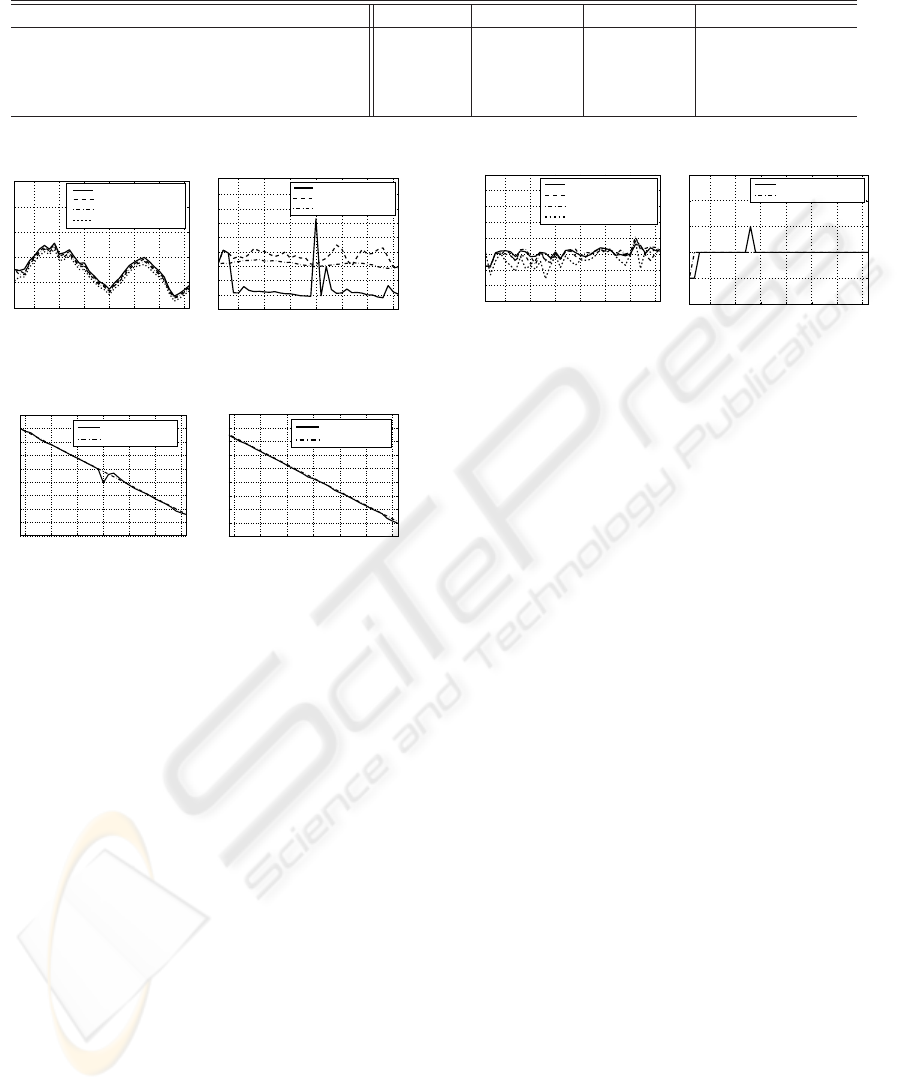
Table 3: Comparison of each calculation time of restoration for 36 frame.
item name Proposed Compared 1 Compared 2 (Belge et al., 2000)
Total iteration number of times 36 71 71 1176
Average iterative number of times per a frame 1 1.97 1.97 32.7
Total calculation time
1:36’41” 3:03’30” 2:57’38” 46:31’34”
Prediction time (within total calc. time)
34” — — —
1 5 10 15 20 25 30 35
1.4
1.6
1.8
2
2.2
2.4
x 10
5
Frame number
Cost Value
Proposed method
Compared method 1
Compared method 2
Belge et al.'s method
Figure 13: Cost value of
the restored images.
1 5 10 15 20 25 30 35
1
2
3
4
5
6
7
8
9
10
x 10
5
Frame number
Cost Value
Proposed method
Compared method1
Compared method2
Figure 14: Cost value of
the initial images.
5 10 15 20 25 30 35
30
40
50
60
70
80
90
100
110
120
Frame number
Position
Predicted value
True value
(a) Vertical direction ¯c
[k]
x
5 10 15 20 25 30 35
30
40
50
60
70
80
90
100
110
120
Frame number
Position
Predicted value
True value
(b) Horizontal direction ¯c
[k]
y
Figure 15: Predicted value of the center of mass (
¯
c
[k]
).
ted the result of the Belge et al.’s method in a dotted
line for reference. In Fig. 13, large differences are
not recognized between each method. In addition, we
show the position of center of gravity of the moving
object in Fig. 15. Fig. 15(a) shows vertical direction
and (b) shows horizontal direction, respectively. We
plotted the true value in a chain line. The horizontal
axis begins with k =4since we did not predict until
k =3. In Fig. 14, the cost value of the predicted
image in our method is almost half of that of the ini-
tial value in other methods in most frames, which the
similar tendency has seen in Table 2. The reason that
the cost values in 1st–3rd, 20th and 22nd frames are
large is thought as follows: for the 1st–3rd frame, the
previous restored image is used for an initial image
directly. As for 20th and 22nd frame, we can see an
larger error in a center of gravity prediction in Fig.
15(a) around these frame, so it is thought that the cost
value increased by influence around the moving ob-
ject domain that took the wrong prediction. However,
since the domain except the moving object domain in
the predicted image of these frames is predicted cor-
rectly, the cost value of the restored image of the pro-
posed method decreased enough by one calculation.
1 5 10 15 20 25 30 35
1.5
2
2.5
3
3.5
4
4.5
5
Frame number
ISNR [dB]
Proposed method
Compared method1
Compared method2
Belge et al.'s method
5.5
Figure 16: ISNR of each
method.
1 5 10 15 20 25 30 35
0
1
2
3
4
5
Frame number
Iteration number of times
Compared method1
Compared method2
Figure 17: Iteration num-
ber of times of the compared
methods.
From Fig. 15(a) and (b), the center of gravity is ap-
proximately correctly predicted in the other frames.
In addition, we show ISNR of the unknown orig-
inal image and the restored image in each frame by
each method in Fig. 16. ISNR of proposed method
is approximately the same as the compared method 1
and 2. However, ISNR of the Belge et al.’s method is
smaller than the other methods in all frames. There-
fore, we understand that there is a similar tendency to
the above 32nd frame in the other frame.
Furthermore, we show the iterative calculation
number of times in the compared methods 1 and 2 in
Fig. 17. The iteration number of times of compared
methods were two or three. In Table 3, we show the
total iteration number of times and calculation time
for the restoration processing of 36 frames. We also
show the prediction time among the calculation time
in the fourth line. The total iteration number of times
of the proposed method were about half of the com-
pared methods 1 and 2, and the similar tendency is
seen about the calculation time. The average predic-
tion time in the proposed method was 1[sec] whereas
the average time of one time iterative calculation was
150[sec]. Therefore, it was shown that the prediction
time in proposed method is extremely smaller than
that of the iterative calculation.
4.1.3 Summary of Simulations
The restoration result of our proposed method has
approximately the same precision quantitatively and
took about half calculation time compared to the com-
pared method 1 and 2. From the subjective evaluation,
the restored images of proposed method have same or
VISAPP 2006 - IMAGE FORMATION AND PROCESSING
78
(a) g
[5]
(a
) f
[5]
rest
(b) g
[40]
(b
) f
[40]
rest
(c) g
[75]
(c
) f
[75]
rest
Figure 18: Restoration results of the real moving image
(5th, 40th and 75th frame).
even better quality than those of the compared meth-
ods. In addition, the large difference was hardly found
by the subjective comparison with the Belge et al.’s
restoration result. Therefore, our result has sufficient
quality enough in addition to the reduction of compu-
tation time. It is concluded that the proposed method
has the effectiveness in the artificially generated de-
graded moving image restoration by quantitative and
qualitative evaluation.
4.2 Experiment for a Real Moving
Image
We show the restoration result using a real original
image. We took a 128×128 pixel moving image
of 256 gradation by an optically blurred fixed CCD
video camera. Since this moving image does not in-
clude motion blur, we applied the degradation model
(8) and executed restoration calculation. The actual
degradation parameters in the moving image are un-
known, but we set as follows experimentally. As for
the optical blur, we supposed a Gauss function of the
fixed variance σ
2
=1.0. As for the disturbance u
[k]
,
we supposed to be a Gaussian noise of SN ratio of
30dB. In Fig. 18, we show degraded images and
restored images of 5th, 40th and 75th frame. Each
image in the right column shows the restored image
f
[k]
rest
corresponding to the degraded image g
[k]
in the
left column. From the experimental result, we can see
that the edges of the moving vehicle and parking cars
are clear compared to its degraded image. Therefore,
we can make sure that the restored images have good
quality by applying above degradation model.
5 CONCLUSION
This paper developed the effective restoration method
for degraded moving image. The dynamics of the
moving image is modeled and a novel calculation al-
gorithm is proposed. From the computer simulation
of the artificially generated moving image, the cal-
culation time was shortened and performances are
increased quantitatively and qualitatively compared
with other methods. Furthermore, we performed
restoration calculation for a real moving image, which
also show a good result, qualitatively.
Although in simulations and experiment, all con-
sidered degradation of the matrix H was optical blur,
it can cope with various degradation factors. In ad-
dition, we can cope with other kinds object motion
by changing the transition matrix T (·). Therefore,
our proposed method can apply to various restoration
processing.
REFERENCES
Banham, M. and Katsaggelos, A. (1997). Digital image
restoration. IEEE Signal Process. Mag., 14(2):24–41.
Belge, M., Kilmer, M., and Miller, E. (2000). Wavelet do-
main image restoration with adaptive edge-preserving
regularization. IEEE Trans. on. Image Processing,
9(4):597–608.
Charbonnier, P., Blanc-Feraud, L., Aubert, G., and Barlaud,
M. (1997). Deterministic edge-preserving regulariza-
tion in computed imaging. IEEE Trans. on. Image
Processing, 6(2):298–311.
Daubechies, I. (1992). Ten Lectures on Wavelets. SIAM.
Geman, D. and Yang, C. (1995). Nonlinear image recov-
ery with half-quadratic regularization. IEEE Trans.
on Image Processing, 4(7):932–946.
Mallat, S. (1989). A theory for multiresolution signal de-
composition: the wavelet representation. IEEE Trans.
on. PAMI, 11(7):674–693.
Osher, S., Ruden, L., and Fatemi, E. (1992). Nonlinear total
variation based noise removal algorithms. Phis. D,
60:259–268.
RESTORATION OF DEGRADED MOVING IMAGE FOR PREDICTING A MOVING OBJECT
79
