
REPRESENTING DIRECTIONS FOR HOUGH TRANSFORMS
Fabian Wenzel, Rolf-Rainer Grigat
Hamburg University of Technology
Harburger Schloßstraße 20, Hamburg, Germany
Keywords:
Parametrization, vanishing points, direction, unit sphere, Hough transform.
Abstract:
Many algorithms in computer vision operate with directions, i. e. with representations of 3D-points by ignoring
their distance to the origin. Even though minimal parametrizations of directions may contain singularities, they
can enhance convergence in optimization algorithms and are required e.g. for accumulator spaces in Hough
transforms. There are numerous possibilities for parameterizing directions. However, many do not account for
numerical stability when dealing with noisy data. This paper gives an overview of different parametrizations
and shows their sensitivity with respect to noise. In addition to standard approaches in the field of computer
vision, representations originating from the field of cartography are introduced. Experiments demonstrate their
superior performance in computer vision applications in the presence of noise as they are suitable for Gaussian
filtering.
1 INTRODUCTION
Many algorithms in computer vision operate with
minimal parameterizations of directions. Some of
their applications can be found in the area of stereo or
multiview geometry, treating directions literally when
estimating rigid body or camera motions. However,
the problem of representing directions is far more
general. In a projective context, it is equivalent to rep-
resenting the projective 2-plane with two components.
A homogeneous coordinate x ∈ P
2
is equivalent to a
globally scaled version λx. Hence, when fixing the
scale such that x =1, the representation problem
also becomes identical to parameterizing unit vectors
or, in other terms, the surface of the unit sphere S
2
.
Minimal parameterizations of homogeneous coor-
dinates are used in optimization algorithms in order
to avoid gauge, i. e. changes in the set of optimized
parameters that have no effect on the value of the cost
function. It has been mentioned that gauge freedoms
introduce ambiguous optima and may lead to slower
convergence (Morris, 2001).
Hough transforms are another example for methods
that require minimal parameterizations, e. g. when lo-
cating vanishing points in an image. A vanishing
point is the intersection of projected lines that are par-
allel in 3D space. In this context, the surface of the
unit sphere S
2
acts as an accumulator space and is
also called Gaussian sphere (Barnard, 1983). This
way, finite or infinite vanishing points can be esti-
mated.
Figure 1 shows an illustration of the vanishing
point location problem. In this example, two pro-
jected lines appear parallel in an image. Thus, the
vanishing point is located at infinity so neither can
it be found in the illustrated figure nor in any larger
Euclidean image. However, the two lines may be
mapped onto great circles on the Gaussian sphere. It
can be seen that their intersection can also be found on
S
2
. In particular, vanishing points at infinity can be
found on its equator if S
2
is oriented such that the po-
lar and the optical axis coincide. The described orien-
tation of S
2
will be assumed for the rest of this work.
Numerous parameterizations of points on S
2
exist
with spherical coordinates (θ, ϕ) being the most ob-
vious one. Here, θ represents the co-latitude, i.e. the
angular deviance from the polar axis, whereas ϕ is
called longitude. It is well-known, however, that pa-
rameterizations may either not be complete or contain
singularities which makes them unsuitable for spe-
cific situations. As an example, spherical coordinates
(θ, ϕ) are singular at the poles as ϕ is not unique for
θ = {0, 180
◦
}.
This paper is organized as follows: After laying out
116
Wenzel F. and Grigat R. (2006).
REPRESENTING DIRECTIONS FOR HOUGH TRANSFORMS.
In Proceedings of the First International Conference on Computer Vision Theory and Applications, pages 116-122
DOI: 10.5220/0001373301160122
Copyright
c
SciTePress
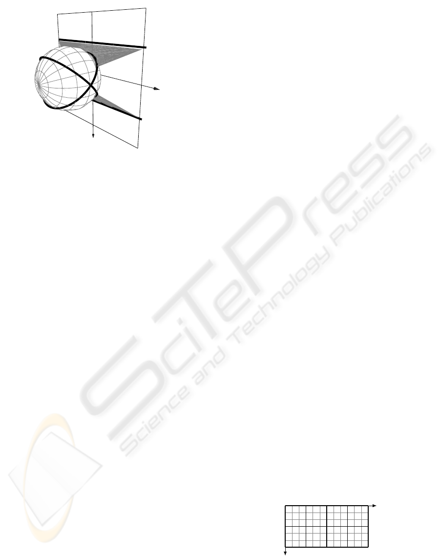
y
x
Figure 1: Gaussian sphere for detecting vanishing points:
Two parallel lines intersect on the equator of S
2
.
some mathematical basics, an overview and compar-
ison of existing parameterizations of S
2
is presented.
Subsequent experiments show that parameterizations
originating from the field of cartography are better
suited for setting up accumulator spaces for Hough
maps in case of noisy input data, not only because of
their numeric properties but also as they may be used
for Gaussian filtering.
2 GLOBAL AND LOCAL
PARAMETERIZATIONS
This section shows that it is impossible to have a
global one-to-one parametrization of S
2
. The follow-
ing details are closely based on (Stuelpnagel, 1964),
in which a similar explanation for parameterizing the
special orthogonal group SO(3) can be found.
The unit sphere S
2
topologically is a 2-dimensional
compact manifold. A global 1-1 parametrization
hence necessarily requires a homomorphism h from
S
2
to the Euclidean space E
2
. A property of homo-
morphisms is that h(U
i
) for an open neighborhood
U
i
of a point i is open in E
2
. Hence, h(I), being the
union of all h(U
i
) for i ∈ S
2
, would still be open.
On the other hand, h(I) describes a continuous map
of a compact space, thus is still compact. As no Eu-
clidean space contains an open compact subset, such
a homomorphism cannot be found.
Parameterizations also fail at singular points on
S
2
that have infinitely many representations. How-
ever, a set of parameter patches, also called an at-
las, circumvents this limitation. An atlas may con-
tain infinitely many parameter patches. In this case,
for a point of interest i, a unique parameter patch
h
i
can be chosen. This technique is also referred to
as a local parametrization (Hartley and Zissermann,
2003). A particular h
i
usually is constructed such
that h(U
i
), the neighborhood of i, does not contain
singular points and has advantageous numerical char-
acteristics. It is interesting to note that local parame-
terizations still may suffer from singularity-like sit-
uations. As an example, (Hartley and Zissermann,
2003) suggests to use Householder transformations
mapping a point of interest i to the origin o and choose
a parametrization that “behaves well” in its vicinity.
However, a Householder transformation does not ex-
ist if i is identical to the origin and is numerically un-
stable if i is close to it (Golub and Loan, 1996). Fur-
thermore, some applications like the Hough transform
explicitly require global parameterizations. There-
fore, local parameterizations cannot be used in every
situation.
A second possibility to circumvent singularities is
to use an atlas with a few parameter patches only
(Faugeras, 1993). Such an atlas is suitable for a
projective setting as representing the complete unit
sphere S
2
is not necessary. As two antipodal points
x and its negative version −x on S
2
are equivalent,
it is sufficient to focus on a hemisphere. Parameter
patches that cover a complete hemisphere exist and
are given in this paper.
3 REPRESENTATIONS OF
DIRECTIONS
Many global parameterizations of directions are men-
tioned in the literature (Snyder, 1987). Some of them
can be found in the field of cartography and have not
been used for Hough transforms before. This section
gives an overview and shows characteristics (see also
table 1). Besides spherical coordinates, we concen-
trate on different azimuthal projections on a hemi-
sphere. Other types are not considered in this work
as they have disadvantegous properties such as sin-
gular points, computational complexity or the lack of
symmetry.
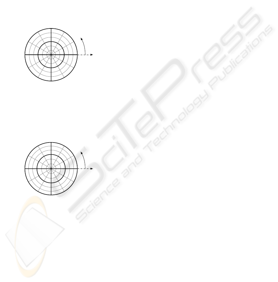
• Spherical coordinates (SPHERICAL):
ϕ
θ
0
◦
180
◦
360
◦
45
◦
90
◦
Even though spherical coordinates yield a singular
point at each of the two poles of S
2
, they are used
REPRESENTING DIRECTIONS FOR HOUGH TRANSFORMS
117
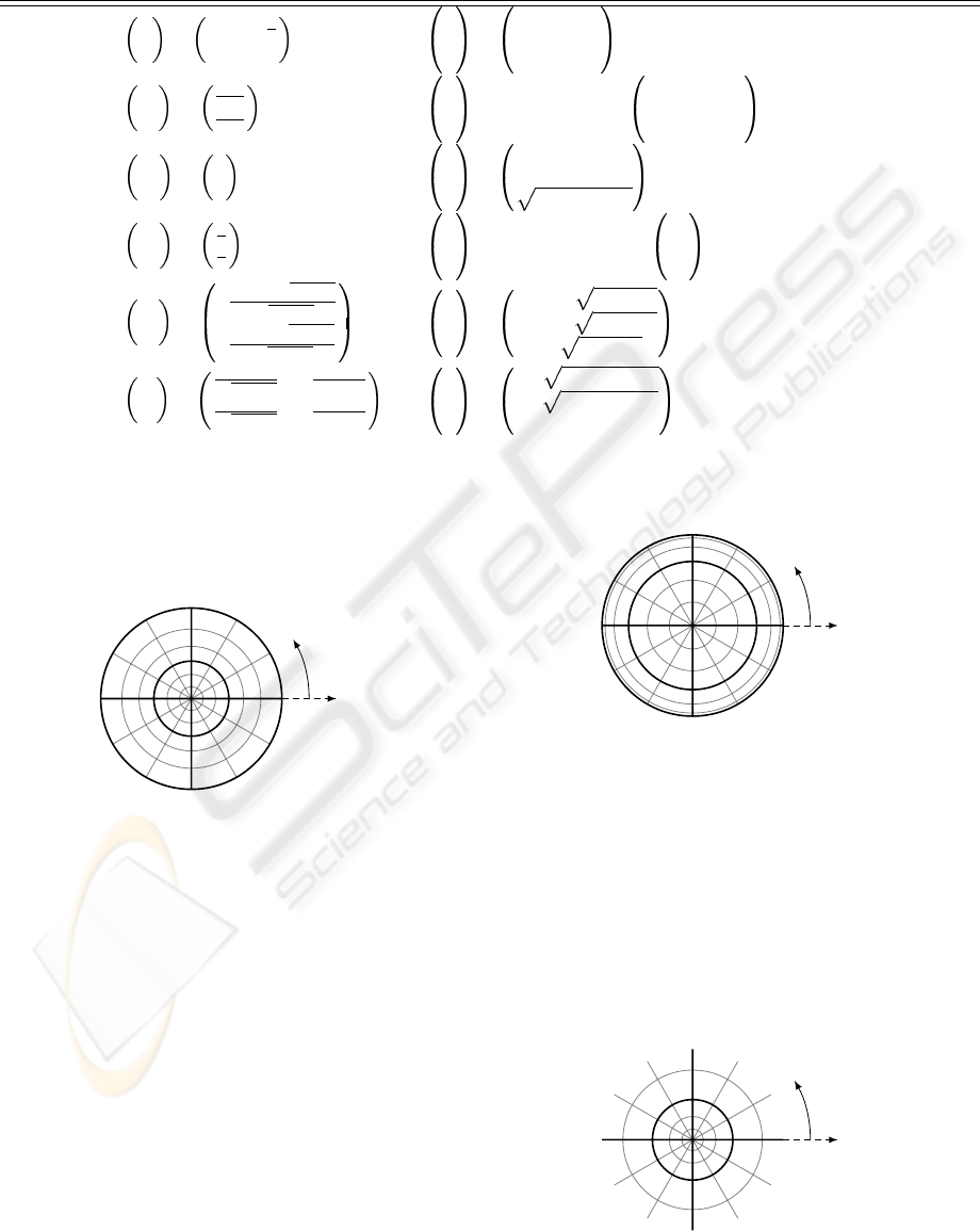
Table 1: Overview of different global parameterizations.
Map from S
2
Map to S
2
(S): Singular points
(U): Non-unique points
SPHERICAL
ϕ
ϑ
=
arctan
y
x
arccos z
x
y
z
=
sin ϑ cos ϕ
sin ϑ sin ϕ
cos ϑ
(S) {x : z =1}
STEREO
x
s
y
x
=
x
1−z
y
1−z
x
y
z
=(x
2
s
+ y
2
s
+1)
−1
2x
s
2y
s
x
2
s
+ y
2
s
− 1
-
ORTHO
x
o
y
o
=
x
y
x
y
z
=
x
o
y
o
1 − x
2
o
− y
2
o
(U) {x : z =0}
GNOMONIC
x
g
y
g
=
x
z
y
z
x
y
z
=(x
2
g
+ y
2
g
+1)
−1/2
x
g
y
g
1
(U) {x : z =0}
EQUI
x
e
y
e
=
x
arcsin
√
x
2
+y
2
√
x
2
+y
2
y
arcsin
√
x
2
+y
2
√
x
2
+y
2
x
y
z
=
x
e
sinc x
2
e
+ y
2
e
y
e
sinc x
2
e
+ y
2
e
cos x
2
e
+ y
2
e
(S) {x : z = −1}
LAMBERT
x
l
y
l
=
x
√
x
2
+y
2
sin
arccos z
2
y
√
x
2
+y
2
sin
arccos z
2
x
y
z
=
2x
l
1 − x
2
l
− y
2
l
2y
l
1 − x
2
l
− y
2
l
1 − 2x
2
l
− 2y
2
l
(S) {x : z = −1}
in many computer vision algorithms (Medioni and
Kang, 2004). Their advantage is the simple geo-
metric interpretation.
• Stereographic projection (STEREO):
ϕ
θ
A standard approach in topology for finding a
parametrization of S
2
is stereographic projection.
Here, the center of projection is located at the north
pole n, the Euclidean plane E
2
as the projection
target is parallel to the equator. Corresponding
points on E
2
and S
2
can be found on the same
ray through n. It is obvious that n itself cannot
be mapped onto E
2
. For computational purposes,
a stereographic projection has the advantage of be-
ing a rational parametrization of directions in R
3
.
Hence, it does not involve trigonometric functions.
• Orthographic projection (ORTHO):
ϕ
θ
By omitting the z-coordinate of a vector in R
3
, the
orthographic projection of a point can be achieved.
This parametrization does not contain singularities,
but an atlas is needed for representing the northern
and southern hemisphere of S
2
uniquely. Its advan-
tage is its computational simplicity given points in
R
3
. It can be seen, however, that azimuthal reso-
lution decreases near the equator. This drawback
is important in section 4 when setting up Hough
maps.
• Gnomonic projection (GNOMONIC):
ϕ
θ
VISAPP 2006 - IMAGE UNDERSTANDING
118
A gnomonic projection in cartography corresponds
to the computation of a Euclidean representation
given a homogeneous vector x ∈ P
2
. Even though
it is rational for points in R
3
, it is not unique
for antipodal points and cannot find a Euclidean
representation of the equator. Moreover, as the
gnomonic projection inverts the process of homog-
enization of point coordinates, computations could
directly be done on the original image. Hence, a
gnomonic projection is suitable for Hough maps
only if points of interest are in a camera’s field of
view.
• Azimuthal equidistant projection (EQUI):
ϕ
θ
An azimuthal equidistant projection yields a 2D po-
lar mapping of spherical coordinates. It preserves
lengths of geodesics through the poles so that Eu-
clidean distances on the map may be used as error
terms.
• Azimuthal Lambertian projection (LAMBERT):
ϕ
θ
The last mapping considered in this paper is az-
imuthal Lambertian projection. It is area preserv-
ing, hence covariance ellipses on S
2
occupy the
same area on the map. However, distances are not
preserved.
4 EXPERIMENTAL RESULTS
Vanishing point detection via intersecting lines on a
Hough map served as an application for evaluating
different parameterizations. We analyzed STEREO,
ORTHO, EQUI and LAMBERT. In section 3 the two
remaining mappings described in this paper have al-
ready been classified not to be suitable for Hough
maps: SPHERICAL yields singular points at the
poles whereas GNOMONIC cannot represent a hemi-
sphere completely. As lines in an original image
are mapped onto curves on the Hough map, a polar-
recursive algorithm has been used for accessing cor-
responding accumulator cells.
In all following configurations, the position and
orientation of intersecting lines has been linearly
transformed prior to Hough transformation such that
the width and height of an input image does not ex-
ceed a horizontal and vertical field of view of 90
◦
.As
a result, the origin of the linearly transformed coor-
dinate system coincides with the center of an image.
Hence, Hough maps conform to the setup illustrated
in figure 1.
A first experiment used synthetic data as input. An
equirectangular point grid has been set up with line
information at each position. Their individual orien-
tations have been chosen such that all lines intersect
at a single location on the x-axis. We examined 10
vanishing points with co-latitudes θ =0
◦
to θ =90
◦
.
Due to symmetry, analysis has been reduced to a sin-
gle longitude ϕ =0
◦
. An example Hough map and
the residual angular error between vanishing point es-
timates and their true positions can be seen in figure
2. In this case errors are only caused by spatial dis-
cretization of the parameter space, i. e. by the finite
resolution of a Hough map. For the used size of 255
× 255 pixels, errors are below 0.5
◦
and could be de-
creased further by increasing the map’s resolution.
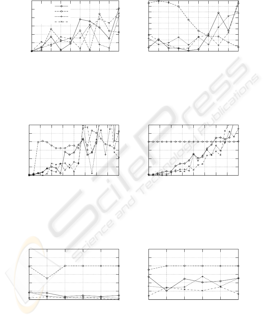
In order to evaluate robustness, we added gaussian
noise with a preset standard deviation σ to all orien-
tation angles. Figure 4 shows results for two noise
levels which demonstrate the effects of the low reso-
lution in θ for ORTHO: Starting from σ =4
◦
, van-
ishing point estimates incorrectly tend to be attracted
by the equator. This problem is caused by the spa-
tial discretization of ORTHO and can be identified in
figure 3(a). Other parametrizations, e. g. LAMBERT,
see figure 3(b), do not suffer from this phenomenon.
The quality of vanishing point estimates is also
affected by the finite number of intersecting lines.
Therefore, in another experiment, we additionally
applied a Gaussian filter with kernel size g to the
Hough map. This approach is contrary to others in
which special techniques like hierarchical (Quan and
Mohr, 1989) or irregular Hough maps are used (Lut-
ton, 1994). Results are shown in figures 5 and 6. It
can be seen that the phenomenon of attractive equator
cells in ORTHO could not be resolved by Gaussian
smoothing. When using other parametrizations, max-
imum residual errors can approximately be halved at
a moderate noise level (figure 6(a)). Best results could
be achieved with EQUI and LAMBERT.
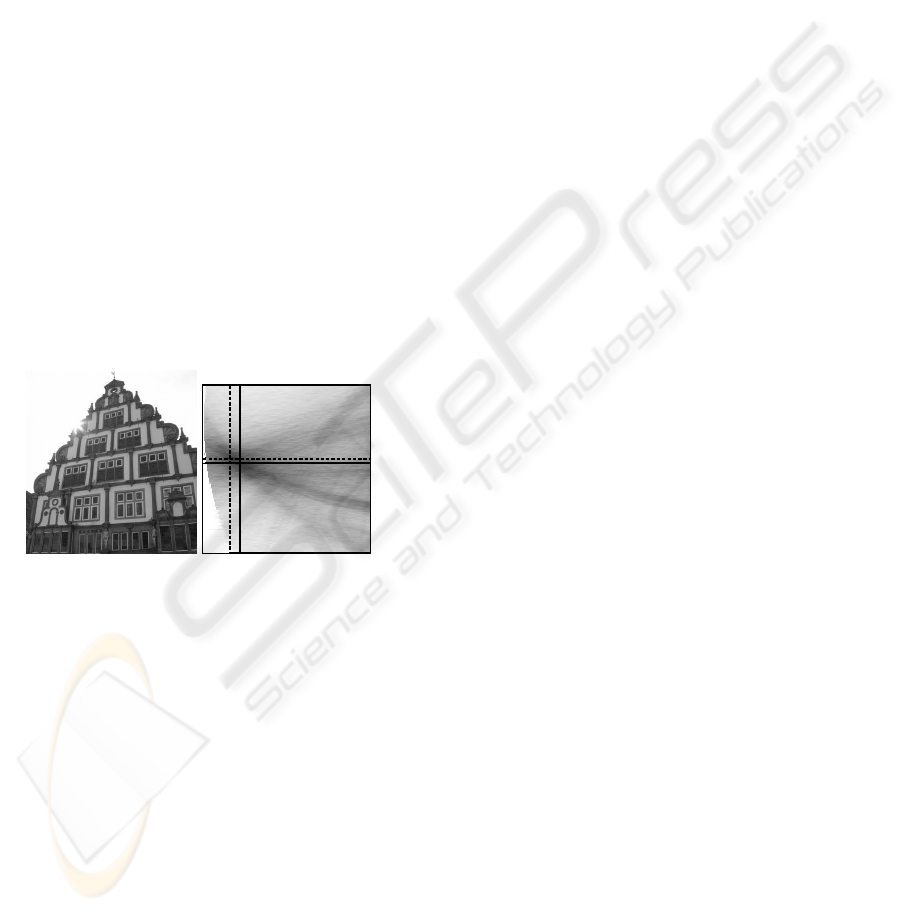
A final, qualitative experiment has been done us-
ing real input data without ground truth. We used
a complex-valued filter for detecting edges (Perona,
1992), (D. Fleet and Jepson, 2000) and used the phase
REPRESENTING DIRECTIONS FOR HOUGH TRANSFORMS
119
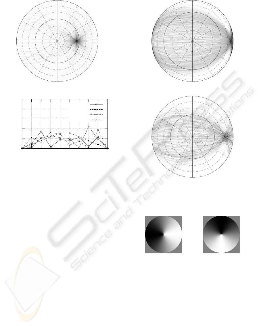
(a)
0
0.2
0.4
0.6
0.8
1
0 102030405060708090
Error (degrees)
Co-Latitude θ (degrees)
STEREO
ORTHO
EQUI
LAMBERT
(b)
Figure 2: (a) LAMBERT map for θ =40
◦
, (b) Residual
errors due to discretization.
of the filter responses as orientation for lines on the
Hough maps. Filter kernels are shown in figure 7.
Figure 8 shows a screenshot as well as a close-up
of of the left vanishing point in the EQUI map. The
marked locations denote point estimates before and
after applying a Gaussian filter. Also in this case, es-
timates can be enhanced by Gaussian smoothing.
5 SUMMARY AND CONCLUSION
We presented parameterizations of the Gaussian
sphere S
2
for detecting directions using Hough trans-
forms. We gave an overview of both known and novel
projections for the field of computer vision. Spherical
coordinates as well as gnomonic projection have been
identified not to be suitable for generating Hough
maps. Experiments show that azimuthal equidistant
and Lambertian projection yield superior results com-
pared to stereographic and orthographic projection.
Finally, we applied a Gaussian filter to Hough maps
that accounts for noise.
(a)
(b)
Figure 3: (a) ORTHO map for σ =6
◦
, (b) LAMBERT map
for σ =6
◦
.
(a) (b)
Figure 7: (a) Real and (b) imaginary part of a complex filter
kernel for edges.
REFERENCES
Barnard, S. T. (1983). Interpreting perspective images. Ar-
tificial Intell., 21:435–462.
D. Fleet, M. Black, Y. and Jepson, A. (2000). Design and
use of linear models for image motion analysis. Inter-
national Journal of Computer Vision, 36(3):171–193.
Faugeras, O. (1993). Three-Dimensional Computer Vision
- A Geometric ViewPoint. MIT Press.
VISAPP 2006 - IMAGE UNDERSTANDING
120
Golub, G. H. and Loan, C. F. V. (1996). MATRIX Compu-
tations. John Hopkins University Press.
Hartley, R. and Zissermann, A. (2003). Multiple View Ge-
ometry. Cambridge University Press, 2. edition.
Lutton, Maitre, L.-K. (1994). Contribution to the deter-
mination of vanishing points using hough transforms.
IEEE Transactions on Pattern Analysis and Machine
Intelligence, 16(4):430–438.
Medioni, G. and Kang, S. B., editors (2004). Emerging
Topics in Computer Vision, chapter Robust techniques
for computer vision. Prentice Hall.
Morris, D. D. (2001). Gauge Freedoms and Uncertainty
Modeling for 3D Computer Vision. PhD thesis,
Robotics Institute, Carnegie Mellon University.
Perona, P. (1992). Steerable-scalable kernels for edge detec-
tion and junction analysis. In European Conference on
Computer Vision, pages 3–18.
Quan, L. and Mohr, R. (1989). Determining perspective
structures using hierarchical hough transform. Pattern
Recognition Letters, 9:279–286.
Snyder, J. P. (1987). Map Projections; A Working Manual.
U.S. Geological Survey, supersedes bulletin 1532 edi-
tion.
Stuelpnagel, J. (1964). On the parametrization of the three-
dimensional rotation group. SIAM Review, 6(4).
(a) (b)
Figure 8: (a) Input image, (b) Close-up of Hough map.
Dashed mark: Estimate before Gaussian smoothing. Solid
mark: Estimate after Gaussian smoothing.
REPRESENTING DIRECTIONS FOR HOUGH TRANSFORMS
121
0
0.2
0.4
0.6
0.8
1
1.2
0 102030405060708090
Error (degrees)
Co-Latitude θ (degrees)
STEREO
ORTHO
EQUI
LAMBERT
(a) Angular errors for σ =2
◦
0
10
20
30
40
50
60
70
80
90
0 102030405060708090
Error (degrees)
Co-Latitude θ (degrees)
(b) Angular errors for σ =40
◦
Figure 4: Effects of different noise levels.
0
5
10
15
20
25
30
0 5 10 15 20 25 30 35 40
Error (degrees)
Angular standard deviation σ (degrees)
(a) Angular errors for g =0pixels
0
5
10
15
20
25
30
0 5 10 15 20 25 30 35 40
Error (degrees)
Angular standard deviation σ (degrees)
(b) Angular errors for g =10pixels
Figure 5: Effects of different Gaussian filter sizes for θ =70
◦
.
0
5
10
15
20
25
30
0246810
Error (degrees)
Gaussian filter kernel size g (pixels)
(a) Angular errors for σ =8
◦
0
5
10
15
20
25
30
0246810
Error (degrees)
Gaussian filter kernel size g (pixels)
(b) Angular errors for σ =20
◦
Figure 6: Effects of different noise levels for θ =70
◦
if Gaussian smoothing is used.
VISAPP 2006 - IMAGE UNDERSTANDING
122
