
INVESTIGATING THE POTENTIAL COMBINATION OF GPS AND
SCALE INVARIANT VISUAL LANDMARKS FOR ROBUST
OUTDOOR CROSS-COUNTRY NAVIGATION
H. J. Andersen, T. L. Dideriksen, C. Madsen and M. B. Holte
Computer Vision and Media Laboratory
Aalborg University, Denmark
Keywords:
Computer vision, Natural landmarks, Visual odometry, Robotics, Stereo vision, GPS, Navigation.
Abstract:
Safe, robust operation of an autonomous vehicle in cross-country environments relies on sensing of the sur-
roundings. Thanks to the reduced cost of vision hardware, and increasing computational power, computer
vision has become an attractive alternative for this task. This paper concentrates on the use of stereo vision
for navigation in cross-country environments. For visual navigation the Scale Invariant Feature Transform,
SIFT, is used to locate interest points that are matched between successive stereo image pairs. In this way the
ego-motion of a autonomous platform may be estimated by least squares estimation of the interest points in
current and previous frame. The paper investigate the situation where GPS become unreliable due to occlusion
from for example trees. In this case, however, SIFT based navigation has the advantage that it is possible to
locate sufficient interest points close to the robot platform for robust estimation of its ego-motion. In contrast
GPS may provide very stable navigation in an open cross-country environment where the interest points from
the visual based navigation are sparse and located far from the robot and hence gives a very uncertain position
estimate. As a result the paper demonstrates that a combination of the two methods is a way forward for
development of robust navigation of robots in a cross country environment.
1 INTRODUCTION
Robotics, control, and sensing technology are today
at a level, where it becomes interesting to investi-
gate the development of mobile autonomous vehicles
to off-road equipment domains, such as agriculture
(Stentz et al., 2002; Bak and Jakobsen, 2004), lawn
and turf grass (Roth and Batavia, 2002), and construc-
tion (Kochan, 2000). Efficient deployment of such ve-
hicles would allow simple, yet boring, tasks to be au-
tomated, replacing conventional machines with novel
systems which rely on the perception and intelligence
of machines.
One of the most challenging aspects of cross-
country autonomous operation is perception such as
in agricultural fields, small dirt roads and terrain cov-
ered by vegetation. Though navigation and position-
ing may be may be achieved using ”global technol-
ogy” such as GPS, the reliability of this is severely
affected by artifacts occluding the hemisphere, such
as trees, buildings etc.. As a results the number and
distribution of the available satellites will be limited
and hence the precision of the position estimate by
triangulation will be degraded and may be subjected
to significant shifts. To account for this drawback of
GPS based navigation it will be necessary to combine
it with locally operating navigation methods.
To perform locally based robot navigation it is
necessary to sense the surrounding environment and
from this derive landmarks or temporal interest points
which may be used for estimation of the robots posi-
tion or ego-motion. This study will focus on the use
of natural landmarks in an outdoor context. Though
markers can be use to support navigation within an
limited area it will always be a solution prone to er-
rors and less generic.
To support the concept of natural landmarks
the scale-invariant feature transform, introduced by
David G. Lowe (Lowe, 2004; Lowe, 1999), will be
used for determination of interest points in an out-
door context. For a more compact representation of
the descriptor the PCA-SIFT method of (Ke and Suk-
thankar, 2004) is used. The SIFT method has pre-
viously with success been used for robot navigation
in an in-door context (Stephen Se and Little, 2002;
Stephen Se and Little, 2005). However, in this con-
text the range of sight for the robot will typically be
limited to within a few meters. In contrast the range
349
J. Andersen H., L. Dideriksen T., Madsen C. and B. Holte M. (2006).
INVESTIGATING THE POTENTIAL COMBINATION OF GPS AND SCALE INVARIANT VISUAL LANDMARKS FOR ROBUST OUTDOOR CROSS-
COUNTRY NAVIGATION.
In Proceedings of the First International Conference on Computer Vision Theory and Applications, pages 349-356
DOI: 10.5220/0001373003490356
Copyright
c
SciTePress
in an outdoor context may be from a few meters to
several hundreds, which gives a very different preci-
sion of landmark based positioning. Looking closer at
the outdoor context it becomes obvious that a combi-
nation of computer vision and GPS based navigation
systems may nicely supplement each other.
In open space away from buildings, trees and other
artifacts GPS will be operating without occlusion of
the hemisphere and hence a good position estimate
may be feasible. In contrast near buildings, trees etc.
the GPS will be subjected to occlusion of the hemi-
sphere and hence the precision and reliability will be
reduced. Looking at a locally operating computer vi-
sion system the situation is the opposite. Near arti-
facts the system will be able to find interest points at
a distance that makes it possible to give a very pre-
cise position estimate. In contrast far from structures
it will be difficult to locate interest points and the dis-
tance to them may be so far that the position estimate
of the robot will be within several meters. So, for once
in a time we are in the happy situation that we have
two technologies that nicely supplement each other.
This paper study the potential of using a binocular
stereo vision setup where interest points are located
and matched in the left and right image pairs, respec-
tively. Next the ego-motion of the robot is estimated
by consecutive matches of interest points in two suc-
cessive frames. The position estimates is compared
with estimates from a differential GPS module.
This paper first outlines the background in terms
of SIFT stereo vision and introduces how this may
be used for estimation of the robots ego-motion. Af-
ter this modeling of stereo error due to quantification
is briefly introduced. The experimental setup is pre-
sented and the experiments investigating the potential
combination of the two navigation approaches is in-
troduced. Finally, the results are discussed and con-
clusions given.
2 MATERIAL AND METHODS
2.1 SIFT Stereo
SIFT is a method for image feature generation for ob-
jects recognition (Lowe, 1999; Lowe, 2004). The
method is invariant in respect to rotation, scale, and
partially to affine transformation, 3D viewpoint orien-
tation, addition of noise and illumination changes. In
general terms the method can be split in to two steps:
• Extraction of interest points
• Description of extracted interest points
An initial set of interest points is found by search-
ing for scale-space extremes. In the SIFT method the
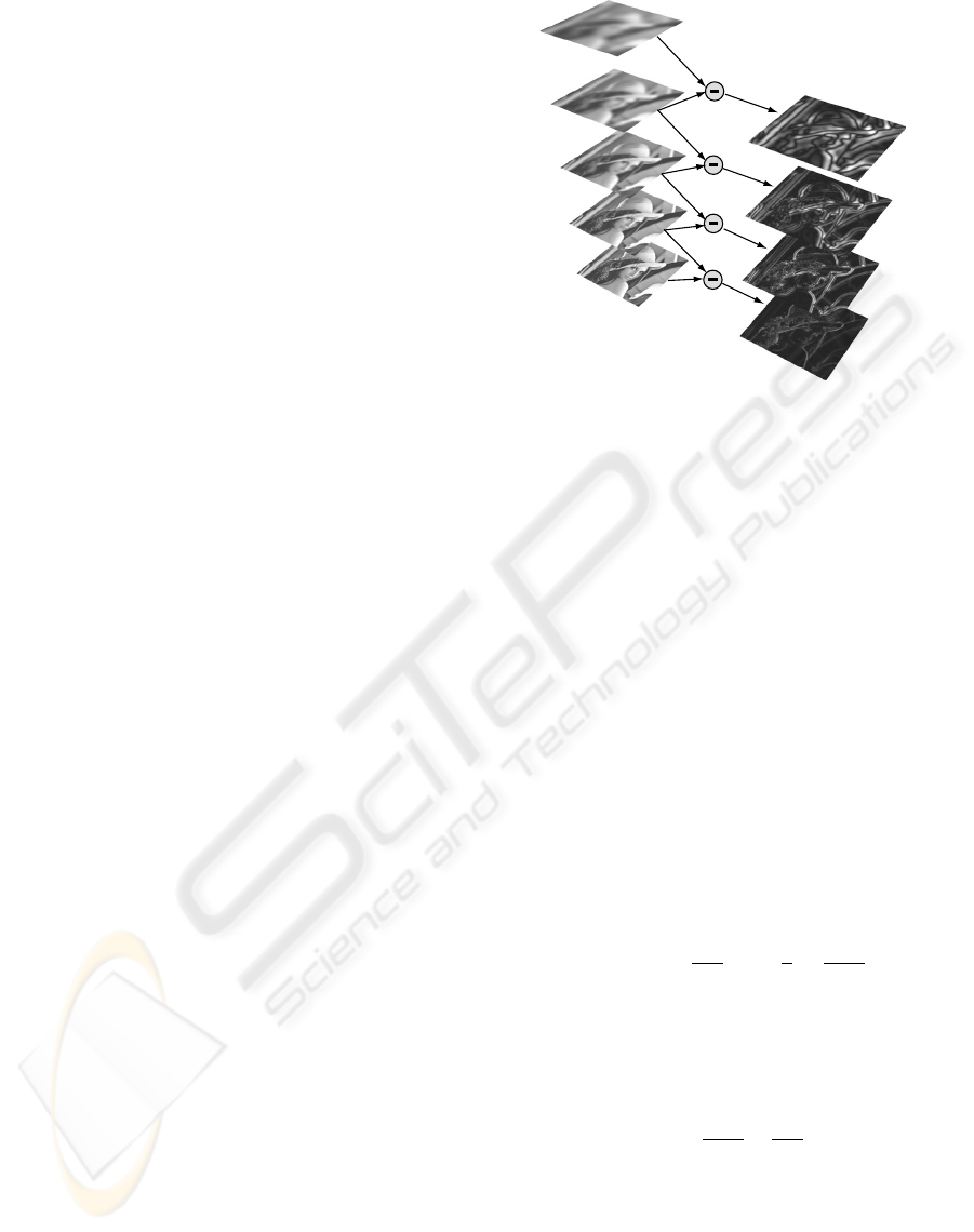
Figure 1: Illustration of Scale-Space and the derived differ-
ent of Gaussian, DoG. The procedure is repeated for every
octave given a DoG pyramid.
continuous scale-space is approximated by a Differ-
ence of Gaussian (DoG) function. In practice the DoG
is generated by smoothing the original image incre-
mentally with a Gaussian kernel and then subtract the
smoothed images at adjacent scales, figure 1. Next
the image is down sampled by a factor two to produce
the next octave in an image pyramid. This is repeated
until the image size is so small that it is impossible to
detect interest points.
The interest points are detected by comparing a
center pixel with its eight neighbors at its own scale
and the nine neighbors at the scale above and below.
For sub-scale and sub-localization of the interest point
a Taylor expansion (up to the quadric term) of the
scale-space function D is centered at the interest point
being evaluated x (Brown and Lowe, 2002):
D(x)=D +
∂D
∂x
T
x +
1
2
x
T
∂
2
D
∂x
2
x (1)
This is especially important for interest points de-
tected at a low resolution. The solution ˆx, is deter-
mined by taking the derivative of the function with
respect to x and setting it to zero:
ˆx = −
∂
2
D
∂x
2
−1
∂D
∂x
(2)
After the sub-scale and sub-localization estimation
each interest point is evaluated with respect to its con-
trast and if it is located along and edge. For the con-
trast the value of the extremum of D(ˆx) is determined
by setting eqn. 1 into eqn. 2. The extremum |D(ˆx)|
is treshold according to a predefined value which it
should be larger that, i.e. there is significant contrast
at the interest point.
VISAPP 2006 - MOTION, TRACKING AND STEREO VISION
350
Interest points located on edges are detected by
evaluation of the principal curvature at the point of
interest. The principal curvature is derived from the
Hessian by the ratio of the squared trace divided by
the determinant of the matrix (Lowe, 2004). Again
interest points are filtered according to a predefined
treshold.
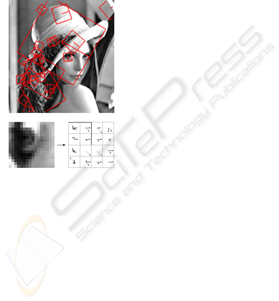
a
Interest point descriptorInterest point region
b
Figure 2: a) Image of Lena with interest points included,
the square around each interest point show the size of the
descriptor region, and the lines in the squares shows the
orientation of the descriptor region. b, left) Detail of the
descriptor region for the interest point at Lena’s left eye ro-
tated according to the regions orientation. b, right) mag-
nitude and orientation of the 4 × 4 descriptor histograms.
Each of them having 8 directions resulting in 128 entries in
the feature vector.
After the selection of interest points the remaining
are described by the orientation in the region around
it and a local descriptor. The orientation of the region
is used to rotate the descriptor region to a consistent
orientation. The 4 × 4 orientation histograms has 8
directions bins in each, will in this way be in the same
order and hence the description of the interest point
will be independent of rotation of the image. Figure
2, demonstrates the SIFT method at the interest point
located at Lena’s left eye. Notice, how the region is
rotated according to the main orientation of it before
the descriptor is formed, figure 2 b. For a more com-
pact and less noise sensitive representation of the fea-
ture with 128 entries in feature vector is projected to
the 36 first eigenvectors of the eigen space introduced
by (Ke and Sukthankar, 2004), also known as PCA-
SIFT.
A match between two interest points is calculated
by the squared distance between them and a similarity
criteria is calculated as the ratio between the best and
second best match. The similarity measure is used for
selection of unique interest points, i.e. a large dis-
tance between the best and second best match. In
the matching procedure only interest points along the
same epipolar lines are considered and between con-
secutive frames the possible ego-motion of the robot
is taking into account.
2.2 Ego-motion Estimation
For calculation of the robots movement between two
consecutive stereo frames the translation and rotation
of the platform has to be estimated. Figure 3, illus-
trates the matching procedure for the stereo and tran-
sient interest points.
For estimation of the translation and rotation the
first part of the two step method by (Matthies, 1989)
is used. The translation and rotation necessary for
alignment of the two 3D points sets, i.e. from the
current and previous frame is estimated by weighted
least square:
Q
c
= RQ
p
+ T
e = Q
c
− RQ
p
− T (3)
SSE = we
T
e
w
j
=(det(Cov
cj
)+det(Cov
pj
))
−1
where Q
c
is the current 3D point set and Q
p
the pre-
vious set and R the rotation matrix, T the translation
vector, SSE is the weighted squared error and w is a
diagonal matrix with the weight w
j
of point j in its
diagonal. The weights are estimated by pooling the
determinants of the 3D points covariances from the
current and previous points sets, last line in eqn. 4.
The points uncertainty are given by modeling of the
stereo error, (see section 2.3). The solution of the ro-
tation R and translation T parameters are given by:
ˆ
R = V
⎛
⎝
10 0
01 0
00det(VU
T
)
⎞
⎠
U
T
(4)
where the vectors V and U are the orthonormal vec-
tors from a SVD of:
K =
j
w
j
˜
Q
cj
˜
Q
pj
T
(5)
INVESTIGATING THE POTENTIAL COMBINATION OF GPS AND SCALE INVARIANT VISUAL LANDMARKS
FOR ROBUST OUTDOOR CROSS-COUNTRY NAVIGATION
351
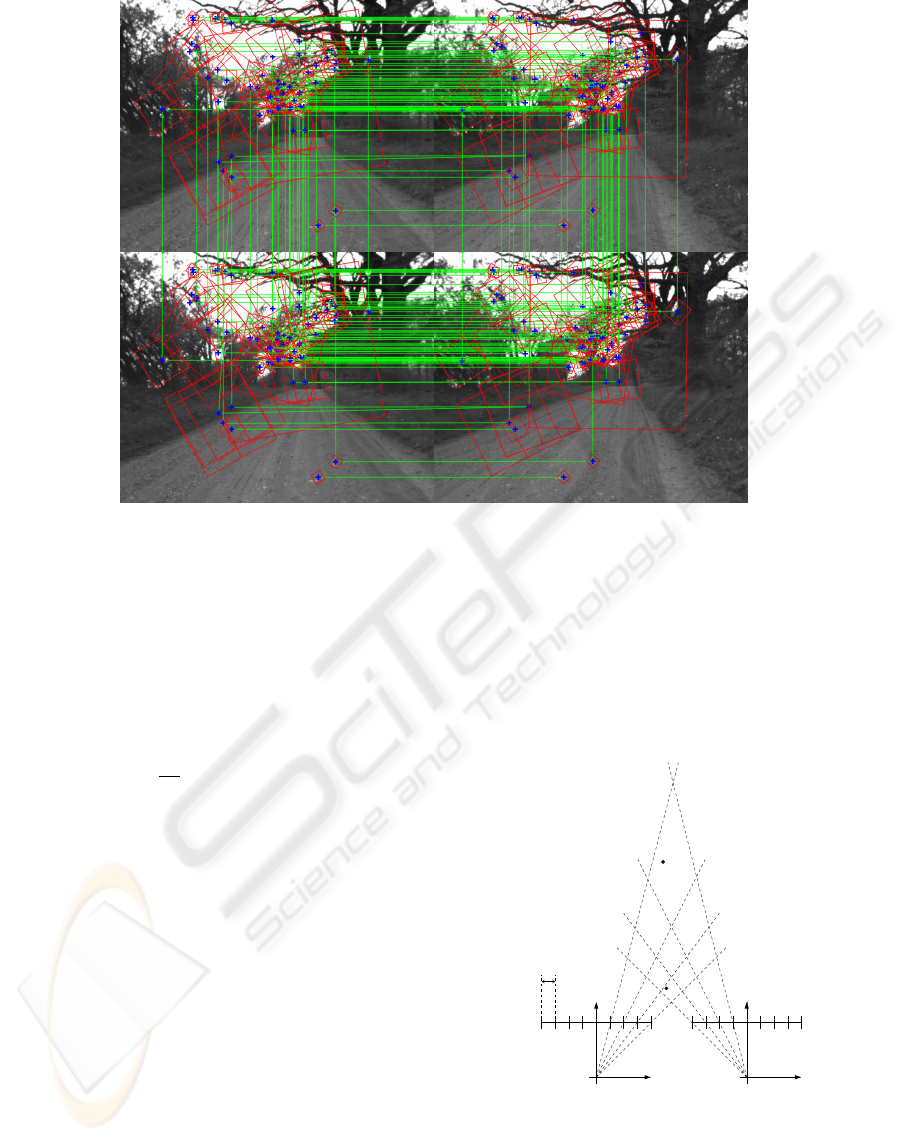
Figure 3: Example of stereo interest point matches and matches between consecutive frames from stereo pair of images from
a linear motion sequence. The top and bottom image pair illustrates stereo corresponding interest points. However, the images
in the top row are from the previous stereo frames, while the bottom row shows the current stereo pair. The superimposed
horizontal green lines denotes stereo matches. Consecutive matched interest points are illustrated by vertical green lines
connecting the two sets of stereo interest points from which the ego-motion of the robot may be estimated.
where
˜
Q
cj,pj
are the two point sets corrected by their
respectively mean values. The translation may now
be estimated by:
ˆ
T =
1
W
[Q
1
−
ˆ
RQ
2
] (6)
where Q
1,2
are the weighted sums of the 3D point sets
and W are the sum of the weights, w
j
.
In the second step of the method the uncertainty
of the 3D points is propagated so it takes the full co-
variance into account. In practice this mean that the
initial estimates of the rotation and translation is cor-
rected for the full covariance structure of the points
location derived from modeling of the stereo error. In
this study this error propagation is not important as
the position estimates is only used for derivation of
the robots ego-motion (visual odometry) and not used
in for example a Kalman filter for fusion with input
from other sensors as GPS, gyro, compass etc. (This
work is in progress).
2.3 Modeling Stereo Error
Due to the quantification of the image sensor an un-
certainty in the reconstruction of the interest points
3D position, is introduced. As illustrated in figure 4
a given point may lie within a polygon. The size of
the polygon is a function of the distance to the stereo
setup and the pixel size.
Left camera Right camera
X
X
ZZ
p
1
2
p
r
l
l
r
P
ixel size x∆
Figure 4: Illustration of the position uncertainty due to
quantification of the image sensors.
For modeling of the uncertainty introduced by the
triangulation the method presented in (Matthies and
Shafer, 1987) is used. This models the polygons by
VISAPP 2006 - MOTION, TRACKING AND STEREO VISION
352
three dimensional Gaussian distributions. For further
detail please consult (Matthies and Shafer, 1987). The
covariances of these distribution are used for estima-
tion of the weights w
j
in eqn. 4.
The depth uncertainty of the triangulation estimates
along the optical axis h
e
is given by the standard for-
mula h
e
=
2h
2
x
Tf−2hx
, where h is the depth, x the
pixel size, T the baseline, and f the focal length. The
function is plotted in figure 5 for the robot setup used
in the experiments.
2.4 Robot Setup
10 20 30 40 50
0
5
10
15
Depth distance h [m]
(2 h ∆ x) /( Tf − 2h ∆ x)
Uncertainty [m]
Figure 5: Uncertainty of the depth estimate along the optical
axis of the stereo setup.
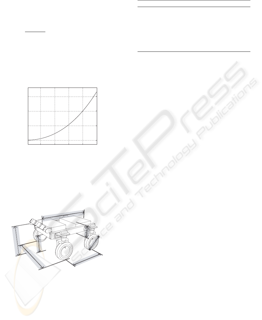
For the experiments the autonomous platform de-
scribed in (Bak and Jakobsen, 2004), will be used
(figure 6). Table 1 summarize the characteristics of
the stereo setup mounted on the platform.
75 cm
100 cm
100 cm
46 cm
60 cm
27 cm
150 cm
Figure 6: The physical dimensions of the API robot.
Images from the stereo setup is synchronously
logged together with corresponding position esti-
mates from a TopCom RTK GPS-module mounted on
robot, so there is a complete correspondence between
the two recordings.
The local coordinate system of the robot has its x-
axis along the baseline of the cameras, the z-axis or-
thogonal to this in the driving direction of the robot.
This gives the bird view plan. The y-axis is perpen-
dicular to this plan, i.e. the elevation plan of the robot.
Table 1: Specifications of the stereo setup.
Parameter Value
Baseline, T 60 cm
Height 75 cm
Focal length, f 8 mm
F-value 1.4
Camera tilt angle 45
◦
Image resolution 640 × 512
Pixel size, x 6.0 x 6.0 µ m
2.5 Experiments
For evaluation of the potential use of computer vi-
sion in combination with GPS three different out-door
experiments was performed. For all experiments the
ground truth of the robots ego-motion is evaluated by
visual comparison of the estimated trajectory by com-
puter vision and GPS. The experiments are designed
so they examine the potentials and drawbacks of the
two methods.
In the first experiment the robot is driving in a lin-
ear motion starting close to a hedge of trees and mov-
ing 19 meters backwards away from this. In the sec-
ond experiment the robot is driving 31 meters on a
gravel road with hedges on either side. The motion
of the robot is oscillating and driven under high con-
trast changes and in way that limits the consecutive
matches between successive frames. The third experi-
ment is a circular motion of 31 meters, which demon-
strates how the vision system looses its capabilities
when it is searching for interest points in an open
country side environment with structures far away. It
also demonstrates how the GPS may suddenly make
abruptly changes when it gets occluded by trees. For
all images the robots motion starts in (0,0). Figure 10,
illustrates examples of images from the right camera
from all three experiments.
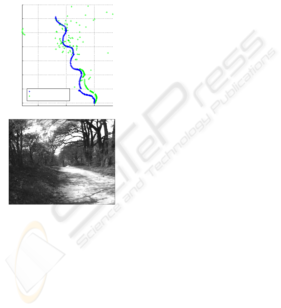
Finally, a fourth experiment (figure 9) is performed,
where the robot is driven in oscillating motion on a
gravel road with large trees on each side covering the
main part of the hemisphere.
3 RESULTS
Evaluation of the experiments is mainly done by vi-
sual comparison of the logged GPS positions and the
ego-motion of the robot. This because the GPS posi-
tions can only partly be used as ”ground truth”.
Figure 7, illustrates the accordance between the
GPS and the position estimates derived from the ego-
motion of the robot of the first three experiments.
For the linear experiment there is good agreement be-
tween the two estimates. From table 2 the robot ends
INVESTIGATING THE POTENTIAL COMBINATION OF GPS AND SCALE INVARIANT VISUAL LANDMARKS
FOR ROBUST OUTDOOR CROSS-COUNTRY NAVIGATION
353
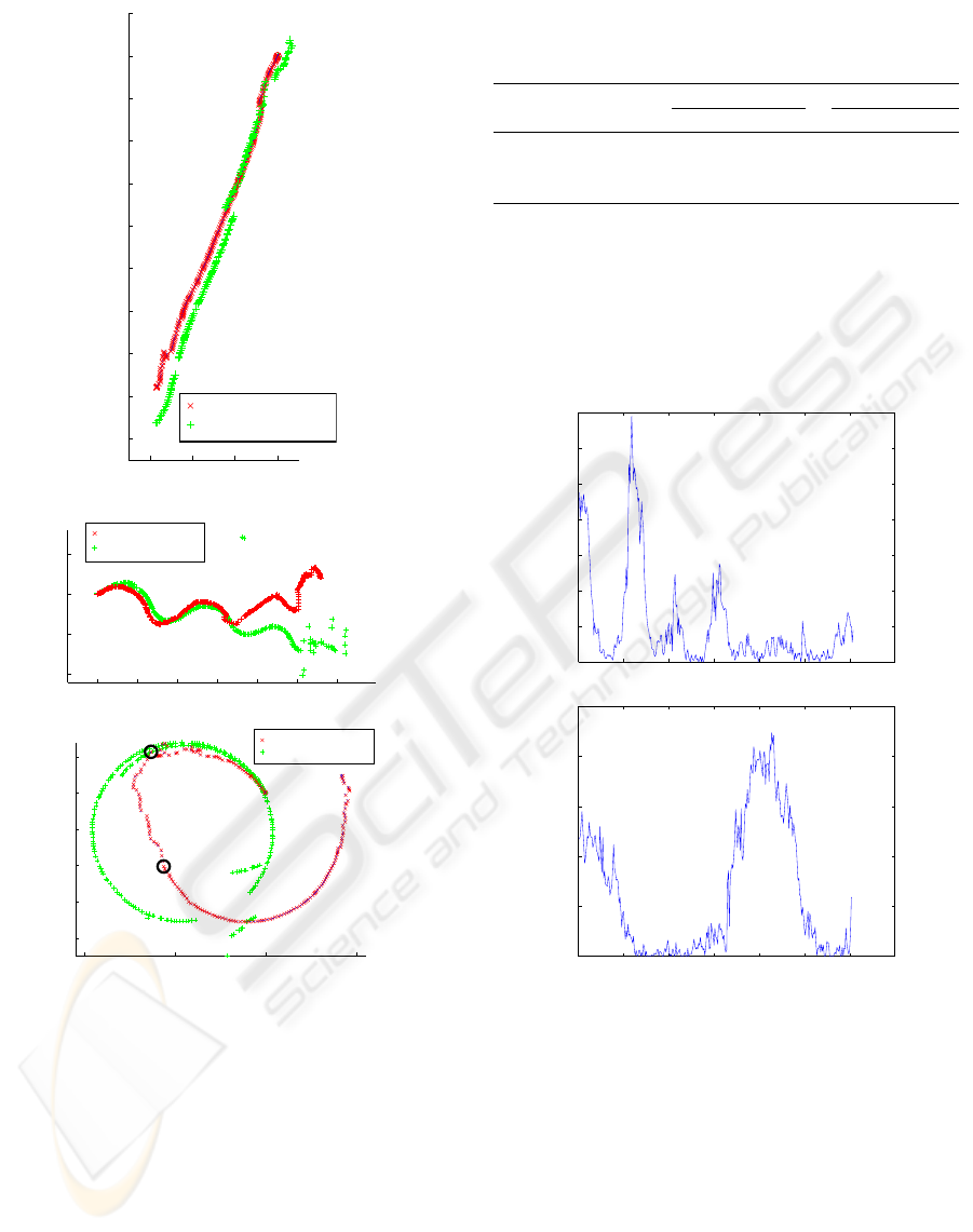
−6 −4 −2 0
−18
−16
−14
−12
−10
−8
−6
−4
−2
0
2
X [m]
Z [m]
System estimate
GPS ground truth
0 5 10 15 20 25 30
−10
−5
0
5
X [m]
Z [m]
System estimate
GPS ground truth
−10 −5 0 5
−8
−6
−4
−2
0
2
X [m]
Z [m]
System estimate
GPS ground truth
Image 65
Image 123
Figure 7: Plot of GPS position estimates (GPS ground truth)
and ego-motion of the robot (System estimate). Top, first
experiment with linear motion, notice the motion is back-
wards. Middle, second experiment with oscillate motion.
Bottom, third experiment with circular motion.
1.67 meters behind the GPS position estimate, which
is within the uncertainty for the stereo setup at a dis-
tance of app. 20 meters, (figure 5).
More complex is the second experiment. In this
the computer vision system is capable of getting good
ego-motion matches until it has moved 15 meters.
Hereafter it loses track mainly due to lack of ego-
Table 2: Summary of the position error development be-
tween GPS and the ego-motion estimates.
Meters Percent
Experiment x z x z
Linear (19m) 0.03 1.67 0.1 8.8
Oscillating (31m) 4.14 -3.55 13.4 10.8
Circular (31m) 12.1 -0.03 39.0 0.1
motion matches according to figure 8 top. This is due
to the oscillating motion of the robot, i.e. there is to
little overlap in the consecutive images for matching
of interest points. Also notice how the GPS gets un-
stable at the end of the sequence.
0 50 100 150 200 250 300 35
0
0
20
40
60
80
100
120
140
Image #
# of temporal matches
0 50 100 150 200 250 300 350
0
50
100
150
200
250
Image #
# of temporal matches
Figure 8: Number of consective matches. Top, second ex-
periment with oscillate motion. Bottom, third experiment
with circular motion.
The circular motion illustrates both the potential
and drawbacks of GPS and visual based navigation.
In the beginning the robot is moving towards and
along the hedge whereafter is field of view at image
65 is changing to the open field until image 123 where
the hedge is appearing in its field view again. Figure
10 bottom, illustrates the sequence. Compared with
the number of consecutive matches (figure 8 it is ob-
vious that between image 65 and 123 there is very
few consecutive matches and hence the ego-motion
VISAPP 2006 - MOTION, TRACKING AND STEREO VISION
354
estimate gets very unstable. For the GPS positioning
estimate there is a abruptly change in the lower right
corner of the circle. However, overlapping the ego-
motion with the GPS position it obvious that the circle
can be closed by fusion of the two position estimates.
01020
0
5
10
15
20
25
30
35
Z [m]
X [m]
System estimate
GPS position
Figure 9: The fourth experiment. Top, accordance between
the position estimate of the robot between the GPS and the
ego-motion estimate. Bottom, example of the surrounding
environment app. half through the sequence.
The last experiment is illustrated in figure 9. This
show the situation where the GPS is significantly oc-
cluded by large trees and hence give a very poor po-
sition estimate, which in many case is several meters
of the visual navigation estimate. The robot moves
in oscillating motion. In the beginning of the se-
quence the hemisphere is only partly occluded. As
the robot moves the trees on either side of the gravel
road gets larger and occludes the hemisphere com-
pletely. In the sequence the computer vision based
ego-motion estimate is able to estimate the motion of
the robot whereas the GPS is significantly disturbed
by the large trees.
4 DISCUSSION
The study presented demonstrates the potential of us-
ing SIFT for localization of interest points in an out-
door environment and further how these may be use
for estimation of a robots ego-motion. Estimation of
the robots location by its ego-motion has been com-
pared with the position estimation from a RTK-GPS
system. The study demonstrates both the advantages
and disadvantages of the two methods but further it
demonstrates that the two methods can nicely supple-
ment each other for robust navigation.
In the study only the ego-motion of the robot has
been used for estimation of it position. Clearly, this
can be extended by inclusion of landmarks that may
be storing in a database and used over several frames.
However, in an outdoor cross-country the number of
landmarks that may be distinct over seasonal changes
of the country side will be very limited. In this respect
the very naive ego-motion estimate only considering
consecutive frames will be a robust method.
Fusion of the ego-motion and GPS positioning es-
timates has not be considered in this study. In further
development this will be a problem to address. The
study, however, illustrates that there is a potential in
fusion of the two methods as they supplement each
other nicely in the situation where the performance
and reliability of one of them is sensitive to the sur-
rounding environment.
5 CONCLUSION
In this study the potential combination of GPS and vi-
sual navigation by use of scale invariant feature trans-
form (SIFT) for detection of interest points in a cross-
country environment has been investigated. The study
demonstrates that if the visual navigation system is
close to artifacts as trees and hedge it is possible to
derive a reliable ego-motion estimate of the robot by
matching of interest points in two consecutive stereo
pairs. On the other hand if the robot is far from struc-
tures the ego-motion of the robot gets unreliable.
In contrast the study demonstrates the sensitively
of GPS when it gets occluded by trees or other arti-
facts. In this situation the position estimate gets un-
reliable and subjected to abruptly changes. However,
this is the situation where the visual navigation sys-
tem is operating with high accuracy. As results and as
demonstrates in the experiments the two methods may
nicely supplement each other in future development
of robust outdoor cross-country navigation systems.
INVESTIGATING THE POTENTIAL COMBINATION OF GPS AND SCALE INVARIANT VISUAL LANDMARKS
FOR ROBUST OUTDOOR CROSS-COUNTRY NAVIGATION
355
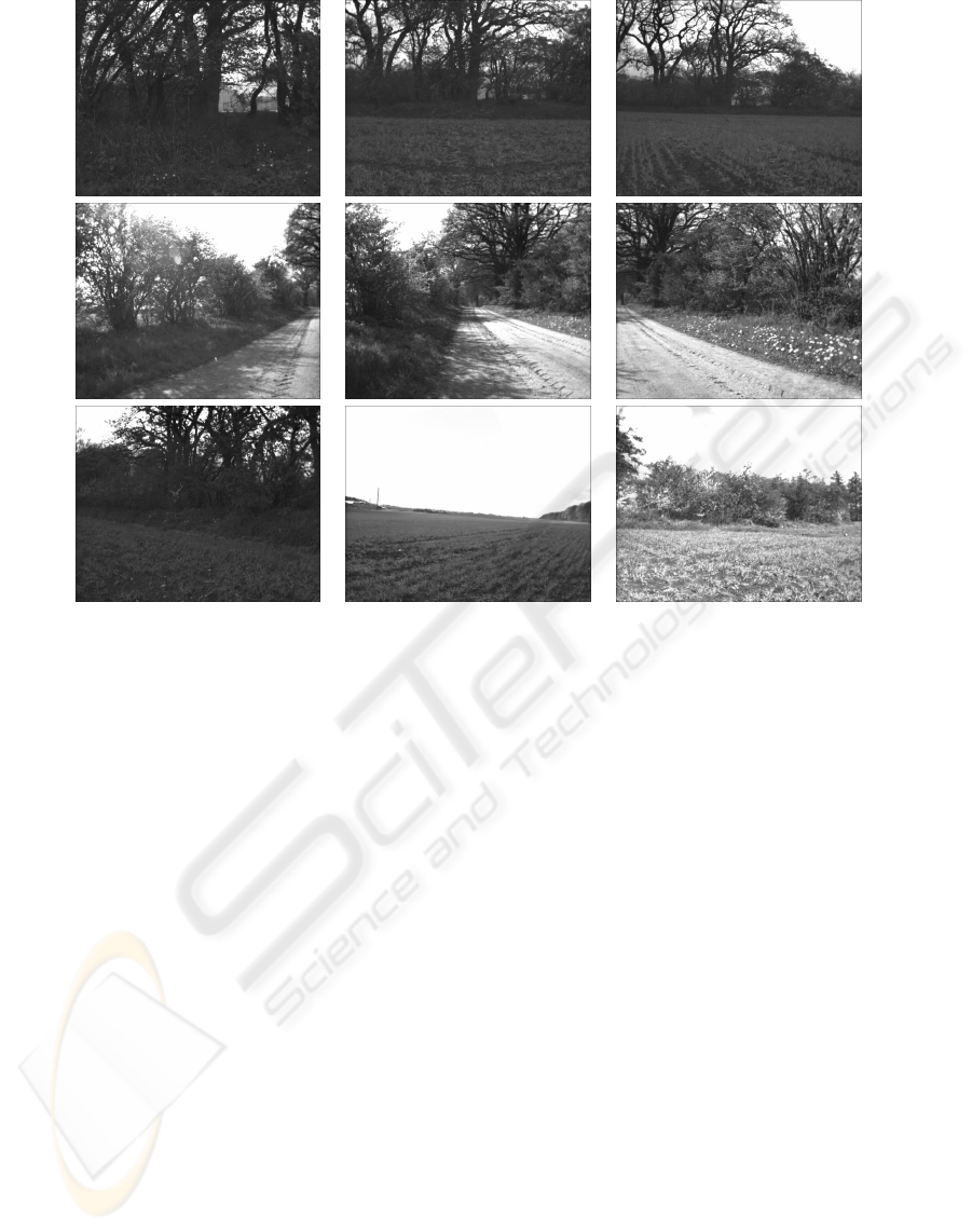
Figure 10: Images from the experiments all images are from right camera in the stereo setup. Top, the first experiments with
linear motion away from a hedge of trees, shown are image 30, 130, and 230. The experiment included 230 images. Middle,
the second experiment with oscillating motion of the robot along a gravel road with hedges on either side, notice the significant
contrast changes. Shown are images 5, 54, and 70. The experiment included 306 images. Bottom, the third experiment with
circular motion at the periphery of a hedge, shown are image 25, 75, and 180. The experiment included 305 images.
REFERENCES
Bak, T. and Jakobsen, H. (2004). Agricultural robotic plat-
form with four wheel steering for weed detection.
Biosystems Engineering, 87(2):125–136.
Brown, M. and Lowe, D. (2002). Invariant features from in-
terest point groups. In Proceedings of the 13th British
Machine Vision Conference, pages 253–262, Cardiff.
Ke, Y. and Sukthankar, R. (2004). Pca-sift: A more dis-
tinctive representation for local image descriptors. In
Computer Vision and Pattern Recognition, volume II,
pages 506–513.
Kochan, A. (2000). Robots for automating construction
- an abundance of research. The Industrial Robot,
27(2):111–113.
Lowe, D. G. (1999). Object recognition from local scale-
invariant features. In International Conference on
Computer Vision, pages 1150–1157.
Lowe, D. G. (2004). Distinctive image features from scale-
invariant keypoints. International Journal of Com-
puter Vision, 60(2):91–110.
Matthies, L. (1989). Dynamic Stereo Vision. PhD thesis,
Carnigie-Mellon University.
Matthies, L. and Shafer, S. (1987). Error modeling in
stereo navigation. Journal of Robotics and Automa-
tion, 3(3):239–248.
Roth, S. A. and Batavia, P. (2002). Evaluating path tracker
performance for outdoor mobile robots. In Automa-
tion Technology for Off-Road Equipment.
Stentz, A. T., Dima, C., Wellington, C., Herman, H., and
Stager, D. (2002). A system for semi-autonomous
tractor operations. Autonomous Robots, 13(1):87–
103.
Stephen Se, Lowe, D. G. and Little, J. (2002). Mobile ro-
bot localization and mapping with uncertainty using
scale-invariant visual landmarks. International Jour-
nal of Robotics Research, 21(8):735–758.
Stephen Se, Lowe, D. G. and Little, J. (2005). Vision based
global localization and mapping for mobile robots.
IEEE Transactions on Robotics, 21(3):364–375.
VISAPP 2006 - MOTION, TRACKING AND STEREO VISION
356
