
MULTIDIRECTIONAL FACE TRACKING WITH 3D FACE MODEL
AND LEARNING HALF-FACE TEMPLATE
Jun’ya Matsuyama and Kuniaki Uehara
Graduate School of Science & Technology, Kobe University
1-1 Rokko-dai, Nada, Kobe 657-8501, Japan
Keywords:
Face Tracking, Face Detection, AdaBoost, InfoBoost, 3D-Model, Half-Face, Cascading, Random Sampling.
Abstract:
In this paper, we present an algorithm to detect and track both frontal and side faces in video clips. By means of
both learning Haar-Like features of human faces and boosting the learning accuracy with InfoBoost algorithm,
our algorithm can detect frontal faces in video clips. We map these Haar-Like features to a 3D model to create
the classifier that can detect both frontal and side faces. Since it is costly to detect and track faces using the
3D model, we project Haar-Like features from the 3D model to a 2D space in order to generate various face
orientations. By using them, we can detect even side faces in real time without learning frontal faces and side
faces separately.
1 INTRODUCTION
In recent years there has been a great deal of inter-
ests in detection and tracking of human faces in video
clips. To recognize people in a video clip, we must
locate their faces. For example, to design a robot ca-
pable of interacting with humans, it is required that
the robot can detect human faces within its sight and
recognize the one it is interacting with. In this case,
the speed of face detection is most important. On the
other hand, when face detection is used in surveil-
lance systems, the speed of face detection is also im-
portant. However it is most important that the system
can detect all faces in the video clips.
Recently, Viola et al. proposed a very fast ap-
proach for multiple face detection (Viola and Jones,
2001), which uses AdaBoost algorithm (Freund and
Schapire, 1996). This algorithm learns a fast strong
classifier by applying AdaBoost to a weak learner.
Then the classifier is applied to sub-images of the tar-
get image, and the sub-images classified into a face
class are detected as faces in the target image. This
approach has two problems:
First, AdaBoost has some problem to use human
face detection. AdaBoost does not consider the re-
liability of the classification result of each sample
with each weak classifier. Furthermore, AdaBoost is
based on decision-theoretic approach, which does not
take the reason of misclassified samples. Therefore,
this algorithm cannot distinguish between misclassi-
fied faces and misclassified non-faces. We will dis-
cuss these problems finely in section 3.
Second, this algorithm can only detect frontal
faces. However the number of frontal faces in video
clips is less than the number of side faces. Addi-
tionally, some algorithms have problems in the ini-
tialization process. Gross et al. (Gross et al., 2004)
use mesh structure to represent a human face, and de-
tect and/or track the face with template matching. In
the initialization process, all mesh vertices must be
marked in every training sample manually. Pradeep
et al. (Pradeep and Whelan, 2002) represent a face as
a triangle, whose vertices are the eyes and the mouth,
and track the face with template matching. In the ini-
tialization process, they need to manually initialize
the parameters of the triangle in the first frame. Ross
et al. (Ross et al., 2004) use eigenbasis to track faces
and update the eigenbasis to account for the intrinsic
(e.g. facial expression and pose) and extrinsic varia-
tion (e.g. lighting) of the target face. In the initializa-
tion process, they need to decide the initial location of
the face in the first frame manually. Zhu et al. (Zhu
and Ji, 2004) use face detection algorithm in the first
frame to initialize the face position. Thereby, they do
not need manual initialization process. However, the
face detection algorithm can detect only a frontal face.
In this paper, we propose an algorithm, which clas-
sifies sub-images to face class or non-face class by
77
Matsuyama J. and Uehara K. (2006).
MULTIDIRECTIONAL FACE TRACKING WITH 3D FACE MODEL AND LEARNING HALF-FACE TEMPLATE.
In Proceedings of the First International Conference on Computer Vision Theory and Applications, pages 77-84
DOI: 10.5220/0001372700770084
Copyright
c
SciTePress
using classifiers. This algorithm does not require
manual initialization process. We substitute Info-
Boost algorithm (Aslam, 2000), which is based on
information-theoretic approach, for AdaBoost algo-
rithm, which is based on decision-theoretic approach.
The reason is to solve the first problem and to im-
prove the precision by using the additional informa-
tion (hypothesis with reliability), which is ignored in
AdaBoost. Additionally, our algorithm does not learn
the whole human face but half of it and maps these
half-face templates to a 3D model. Then the algo-
rithm reproduces the whole-face template from the
3D model with some angle around the vertical axis.
As a result, we can detect faces, which are even ro-
tated around the vertical axis, by using the reproduced
whole-face templates.
2 HAAR-LIKE FEATURES
In this paper, Haar-Like features are used to classify
images into a face class or a non-face class. Some
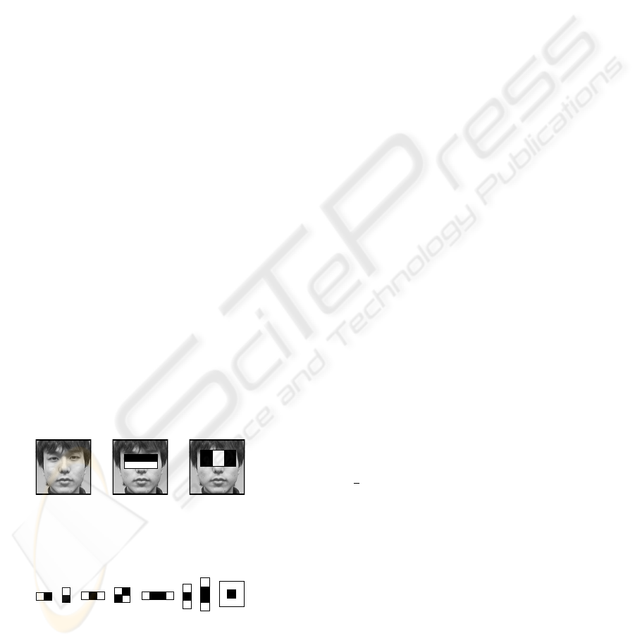
samples of Haar-Like features are shown in Figure 1.
Basically, the brightness pattern of the eyes distin-
guishes the face from the background. (a) is an orig-
inal facial image. (b) measures the difference in
brightness between the region of the eyes and the re-
gion under them. As is shown in (b), the brightness
of the eyes is usually darker than the skin under them.
(c) measures the difference in brightness between the
region of the eyes and the region between them. As is
shown in (c), the eyes are usually darker than the re-
gions between them Thus, an image can be classified
as a facial or a non-facial class based on the brightness
pattern described above. These features are generated
from feature prototypes (Figure 2) by scaling these
prototypes vertically and horizontally.
(b)(a) (c)
Figure 1: Feature Example.
(a) (b) (c) (e) (f) (g) (h)(d)
Figure 2: Feature Prototypes.
We calculate the average brightness B
b
, B
w
in the
black region and the white region of the features, and
use their difference (F = B
b
− B
w
) as a feature
value. Then we use these feature values as parame-
ters to classify images into a face class or a non-face
class. For example, when a feature of Figure 1(b) is
applied to a true human face, F is too large. Accord-
ingly, we decide the threshold of the classification and
classify images according to the feature value F , if it
is larger or smaller than the threshold. If F is larger
than the threshold, the image is classified into a face
class. If F is smaller than the threshold the image is
not a human face.
Viola et al. use feature prototype (a)-(d) shown in
Figure 2. We use four additional prototypes (e)-(h).
Prototype (e) will measure the difference in bright-
ness between the region of the mouth and its both
ends. The black region of prototype (e) will match
the region of the mouth, and the white regions will
match both ends of the mouth. The black region of
prototype (f), (g) will match the region of the mouth
(the eyes), and the white regions will match the top
and bottom of the region of the mouth (the eyes). The
black region of prototype (h) will match the region
of the eye (the nose or the mouth), and the white re-
gion will match the region around the eye (the nose or
the mouth). Therefore, these feature prototypes will
be effective to classify images to face and non-face
classes.
If we add these effective feature prototypes like (e)-
(h), the learning time will be somewhat increased,
while the speed of classification will be improved. If
we add some compound feature prototypes, the time
of classification will be decreased. For example, fea-
ture prototype (e) can be considered as the prototype,
which is made by combining the prototype (a) twice.
In the region where the feature prototype (e) can be
used, we need to calculate twice for the value of the
feature generated from prototype (a). But now we
need only one calculation for the value of the feature
generated from the prototype (e). So the time com-
plexity is decreased for these regions, and the detec-
tion time can be reduced. In this case, if we need t
seconds to face detection with prototype (a), we only
need
1
2
t second to face detection with prototype (e).
3 APPLYING INFOBOOST
Classification with Haar-Like features is fast, but it
is too simple and its precision is not very impressive.
Hence, we apply a boosting algorithm to generate a
fast strong classifier. AdaBoost is a most popular
boosting algorithm.
3.1 AdaBoost
AdaBoost assigns the same weight to all training sam-
ples and repeats learning by weak learners while up-
VISAPP 2006 - IMAGE UNDERSTANDING
78

dating the weights of the training samples. If the weak
classifier generated by the weak learner classifies a
training sample correctly, the weight of the sample in-
creases. If the weak classifier misclassifies a training
sample, the weight of the sample decreases. By this
repetition, the weak learner becomes more focused
on the sample, which is difficult to classify. At last,
by combining these weak classifiers with the voting
process, AdaBoost generates one strong classifier and
calculates the final hypothesis for each sample. The
voting process evaluates results of weak classifiers by
majority decision and decides the final classification
result. Nevertheless, we use InfoBoost to increase the
precision of the classifier because there are two prob-
lems in AdaBoost.
Weak classifiers generated in the AdaBoost pro-
cess do not consider the reliability of the classifica-
tion result for each sample. Hence, the classifiers
which classify the sample with high reliability and
those which classify the sample with low reliability
are combined without any consideration of their reli-
abilities.
For example, assume that nine weak classifiers are
generated in the AdaBoost process. If four of them
classify a sample into a face class with 95% accu-
racy, and five of them classify the same sample into
a non-face class with 55% accuracy, the image will
be classified into a non-face class. If we introduce the
reliabilities of these classifications, the sample should
have been classified into a face class.
Another problem is that AdaBoost is based on
decision-theoretic approach. AdaBoost algorithm
only deals with two cases, whether the classification
is true or false, when the weights are updated. But
actually there are the following four cases to be con-
sidered.
• A face image classified into a face class.
• A non-face image classified into face class.
• A face image classified into a non-face class.
• A non-face image classified into a non-face classD
The incidences of these classifications are not always
the same. For example, in a certain round of Ad-
aBoost, if the number of misclassified face images
and the number of misclassified non-face images are
nearly equal, all we are required to do is to decrease
the weights of correctly classified samples and to in-
crease the weights of incorrectly classified samples.
In contrast, if the number of misclassified non-face
images is larger than the number of misclassified
face images, the misclassified non-face images will
be classified correctly in the next round or later, al-
though the misclassified face images may not be cor-
rectly classified. The reason is that AdaBoost does
not take care of the difference of two misclassifica-
tion cases. Therefore, we should not depend only on
the classification result (true or false) for weight up-
dating, but we must also consider the correct classes
(positive or negative). When we update the weight of
each sample image we must consider these four cases
separately.
3.2 InfoBoost
In this paper, we consider the two problems of Ad-
aBoost and use InfoBoost algorithm, which is a mod-
ification of AdaBoost. We propose three points where
InfoBoost and AdaBoost differ:
First, InfoBoost repeats the round T times (t =
1, · · · , T ) in the learning process. In round t, weak
hypothesis h
t
is shown by h
t
: X → R. The hypothe-
sis represents not only the classification result but also
the reliability of the classification result. In order to
make it easy to handle, we restrict the region of hy-
pothesis h
t
to [−1, +1]. The sign of h
t
represents the
class of prediction (−1 or +1), and the absolute value
of h
t
represents the magnitude of reliability. For ex-
ample, if h
1
(x
1
) = −0.8, h
1
classifies the sample x
1
into the class −1 with the reliability value 0.8.
Second, the accuracy of negative prediction α
t
[−1]
and the accuracy of positive prediction α
t
[+1] are cal-
culated. These values are calculated using equation
(1), (2).
α[−1] =
1
2
ln
1 + r[−1]
1 − r[−1]
(1)
α[+1] =
1
2
ln
1 + r[+1]
1 − r[+1]
(2)
r[−1] =
P
i:h(x
i
)<0
D
t
(i)y
i
h
t
(x
i
)
P
i:h(x
i
)<0
D(i)
(3)
r[+1] =
P
i:h(x
i
)≥0
D
t
(i)y
i
h
t
(x
i
)
P
i:h(x
i
)≥0
D(i)
(4)
y
i
is the correct class of the sample x
i
, and D
t
(i) is
the weight of the sample x
i
in round t. α
t
[−1] and
α
t
[+1] reflect the magnitude of reliability and the pre-
cision of classification for each sample. If hypoth-
esis h
t
classifies x
i
into the class −1, α
t
(h
t
(x
i
)) is
α
t
[−1]. If hypothesis h
t
classifies x
i
into the class
+1, α
t
(h
t
(x
i
)) is α
t
[+1].
Third, the weight D
t
is updated according to equa-
tion (5)
D
t+1
(i) =
D
t
(i) exp(−α
t
(h
t
(x))y
i
h
t
(x
i
))
Z
t
(5)
Z
t
is a normalization factor. It is chosen in a way
that
P
i
D
t+1
(i) = 1. By executing this operation,
the weight of the sample classified correctly with hy-
pothesis h
t
(x
i
) is decreased, while the weight of the
sample classified incorrectly with hypothesis h
t
(x
i
)
is increased.
MULTIDIRECTIONAL FACE TRACKING WITH 3D FACE MODEL AND LEARNING HALF-FACE TEMPLATE
79
We repeat these processes T times, and calculate
the final hypothesis H with the T weak hypotheses.
Then we take a weighted vote among hypotheses us-
ing α
t
(h
t
(x
i
)) as weight. If the result of voting is a
negative value, we output −1 as the final hypothesis,
and if the result of voting is a positive value, we out-
put +1 as the final hypothesis.
When we apply InfoBoost to weak learners, it is
necessary to show how correct the classification re-
sults of training samples are. We calculate the feature
value for each training sample, the difference d of the
feature value f , and the threshold t (d = f − t). The
sign of difference f represents the classification re-
sult. If the absolute value of d is too small, the feature
value f is near the threshold d. The sample classified
+1 might be classified −1, so it is not trusty. Con-
versely, if the absolute value of d is too large, the clas-
sification result is trusty. Obtaining the difference be-
tween feature value and threshold, we can express the
classification result and its reliability for each sample.
Therefore, we use the difference between the feature
value and the threshold as the classification result with
evaluation of reliability.
Because InfoBoost is based on information-
theoretic approach, it does not only have the benefit of
the improvement of the classification’s precision, but
also it can provide some flexibility for the classifier.
For instance, in surveillance systems, we must detect
all human faces while it is allowed to mis-detect few
non-faces as faces. On the other hand, if a surveil-
lance system of a building cannot detect some faces
and those people commit a crime in the building, we
cannot place their faces on the wanted list. Thus the
surveillance system which cannot detect some human
faces is not useful.
By increasing the weight of face samples classified
into non-face class, the learning process focuses more
on the misclassified face image and the final classifier
will be able to detect almost all human faces more
accuratly. Hence, we can adapt classifiers for surveil-
lance systems by adjustment of weights of samples.
InfoBoost can bias the classification basis based on
the importance according to the four cases (face clas-
sified into face, face classified into non-face, non-face
classified into face, and non-face classified into non-
face) by biased the rules of updating weight.
4 3D MODEL AND LEARNING
HALF-FACE TEMPLATE
In video clips, the probability of having complete
frontal faces is not high. Most of them are side faces.
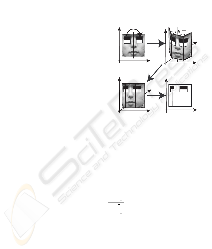
Consequently, we map the classifier learned from fa-
cial features to a 3D model (Figure 3(a)(b)). The
3D model consists of three areas (r), (c), (l) (in Fig-
ure 3(b)). (r) is the right part of the 3D model, (c)
is the center part of the 3D model, and (l) is the left
part of the 3D model. These parts of the 3D model
are plane faces, and their joint angles are
π
4
in Fig-
ure 3(b). By using this 3D template, the classifier will
be able to detect not only frontal faces but also side
shots of faces.
(a) Feature in 2D
(b) 3D-Model
Mapping
Reverse Feature
(d) Rotated Feature
in 2D
Projection
(c) Rotated Feature
with 3D-Model
Rotate
(r)
(c)
(l)
(r)
(c) (l)
(r)
(c) (l)
4
4
Figure 3: Feature Projection.
If we use 3D model in face detection, time com-
plexity is increased and detection speed is decreased,
because the calculation of 3D model is time consum-
ing. Therefore, we create a new classifier by rotating
the 3D model around the vertical axis and by project-
ing the 3D model classifier back to 2D again (Fig-
ure 3(c)(d)). By using these classifiers, we do not
need calculation of 3D model in the detection process,
so the time complexity does not increase much.
If the rotation angle is θ (positive for clockwise
rotation), the width w
r
of area (r) is modified to
cos(θ−
π
4
)
cos
π
4
w
r
, the width w
c
of area (c) is modified to
cos(θ)w
c
, and the width w
l
of area (l) is modified to
cos(θ+
π
4
)
cos
π
4
w
l
. We execute these processes in every 30
degrees of rotation angle and use these classifiers in
parallel to prevent the increase of time complexity.
But, there is a self-occlusion problem. When the
3D model is rotated enough, (r) or (l) of the 3D model
is occluded by (c), and some feature rectangles in 3D
model may be hidden and we cannot use these fea-
tures. If the 3D model in Figure 3 is rotated in clock-
wise direction enough, the part of the feature at the
right eye in (r) will be hidden and we cannot use this
feature. Hence, we do not use whole faces but use
half-faces as learning samples.
VISAPP 2006 - IMAGE UNDERSTANDING
80

Furthermore, because of the face symmetry, we ex-
press the whole face by combining reversed facial fea-
tures with the original ones (Figure 3(a)). Therefore,
even if the 3D model is rotated, we can use all features
of either the right half or the left half of the face.
Additionally, because of learning half-faces, we
can be free from the different illumination states be-
tween left and right faces. We use the right side and
reversed left side of whole face samples as the half-
face samples, thus the half-face classifier is robust to
the difference between the left and the right of the
faces.
The classifier generated from the boosting algo-
rithm is a set of weak classifiers using Haar-Like fea-
tures. Each weak classifier consists of the following
elements: coordinates of the reference points, width
and height of the white and black rectangles of Haar-
Like feature, and the threshold of Haar-Like feature.
In Figure 4, P
w
is the reference point of the white
rectangle of Haar-Like feature, and P
b
is the reference
point of the black rectangle of Haar-Like feature. The
coordinates of these rectangles are shown as X
w
, X
b
,
Y
w
, Y
b
, and widths and heights of these rectangles are
shown as W
w
, W
b
, H
w
, H
b
.
0
x
y
Hw
Hb
Wb
Ww
Pw
Pb
Xb
Yw
Yb
Xw
Figure 4: Parameter of Haar-Like Feature Rectangle.
Therefore, the features are easily mapped to the 3D
model shown in Figure 3(b). Then, we confine that
3D model can only be rotated around the vertical axis,
as a result feature rectangles are scaled only in hori-
zontal axis (see Figure 3(a) and (d)). Therefore, the
weak classifier generated by projecting the features
from 3D model to 2D can be transformed by mov-
ing, expanding and/or shrinking the Haar-Like feature
rectangles of the original weak classifier horizontally.
5 EXTENSION OF CASCADING
Cascading is the algorithm to reduce the time com-
plexity of classification. Cascading algorithm gener-
ates the cascade of small classifiers by dividing the set
of weak classifiers into some subsets. The first classi-
fier of the cascade classifies all samples. The samples
classified into negative samples are not passed to the
following classifiers. By doing this, cascading algo-
rithm reduces the number of samples to be evaluated
and the time complexity of classification. To generate
each weak classifier, the learning process is executed
with a constrained condition (T P > minT P ) while
F P < maxF P . True positive rate T P and false pos-
itive rate F P are calculated as follows:
T P =
number of correctly classified faces
total number of faces
(6)
F P =
number of misclassified non-faces
total number of non-faces
(7)
minT P and maxF P are parameters of the learning
process. We execute learning process with minT P =
0.999 and maxF P = 0.4.
We extend boosting and cascading process in the
following three points to reduce the time complexity
of face detection and learning time.
• The configuration of the cascading.
• The termination condition of the learning process.
• The number of samples used in AdaBoost process.
First, when we use half-face templates, we must
evaluate them separately and aggregate these evalu-
ation results. As is shown in Figure 5, the classifier
consists of two cascades. In this case, both of the cal-
culations of these cascades are executed every time.
However, when the target sample is rejected in an
early stage in one of these cascades, the calculation of
another cascade makes no sense. Therefore we com-
bine these cascades as shown in Figure 6 to reduce the
unnecessary process. By using this new cascade, the
unnecessary process is avoided. If the target sample
is rejected in an early stage on one of the cascades,
the calculation on another cascade is stopped imme-
diately.
Second, when we use half-faces as learning sam-
ples, characteristic features of a face are much fewer
than those of whole face samples. If we use whole
faces as learning samples, we can use all features
learned from the whole face. However we cannot use
some of these features (for example, the feature in
Fig 1(b), (c)), because we use half-faces as learning
samples. Thereby, we will use some new features that
can be applied to half-faces to substitute for the fea-
tures that we cannot use here. These new features are
more delicate, hence their number is larger than that
of the features that can only be applied to the whole
faces. As the tradeoff, the speed of face detection will
be decreased, because a simple feature based on the
whole face is replaced by several small features based
on the half-face. Accordingly, in the learning process,
if precision of the classifiers is enough to detect faces,
we finish the learning process. As the learning pro-
cess makes progress, the face detection rate will hit a
peak. Simultaneously, the number of features which
are necessary to classify both positive and negative
MULTIDIRECTIONAL FACE TRACKING WITH 3D FACE MODEL AND LEARNING HALF-FACE TEMPLATE
81
True True
True
False False False
right half of
part images
input data classified into a non-face
True
. . .
input data
classified
into a face
True True True
False False False
left half of
part images
True
. . .
part
images
split AND
TrueFalse
Figure 5: Two Classifier Cascades.
True True
True
False False False
right half of
part images
input data classified into a non-face
. . .
input data
classified
into a face
True
False False False
left half of
part images
. . .
part
images
split
input data classified into a non-face
. . .
True True
Figure 6: Combining Two Classifier Cascades.
samples will become larger. For this reason, we stop
the process when both the precision and the recall are
larger than 0.95.
Third, in learning process, we must use many sam-
ple images to detect almost all faces. However, when
we use many sample images, the time complexity of
the learning process is very huge. Therefore, we use a
subset of all samples to generate each small classifier.
These samples are selected by random sampling.
Random sampling is a sampling algorithm which
pick out some samples from all samples randomly
without overlapping. Random sampling is used where
we cannot evaluate all samples (for example, market-
ing). The probability of each sample to be picked out
is same. Therefore, the selected samples are minia-
ture versions of all samples, and the learning result
with selected samples will be similar to that with all
samples.
We must decide the total number of selected sam-
ples. We decide the number based on “Chernoff
bound” (Chernoff, 1952). The number of selected
samples n are defined by inequality (8).
n >
1
2ǫ
2
ln
2
δ
(8)
According to “Chernoff bound”, if the above inequal-
ity is satisfied for any ǫ (0 < ǫ < 1) and any δ
(0 < δ < 1), the number of sample n is enough for
classification. We use this inequality as ǫ = 0.05,
δ = 0.01, and get the minimum n = 1060. Thus we
select 530 positive samples and 530 negative samples
in each stage to generate small classifiers.
6 EXPERIMENTS
We performed five experiments. We use a window
to extract sub-images from the original image. Mini-
mum size of the window is 38x38 pixels, translation
factor is 0.5 * window size and scale factor is 1.2.
First, we compare the precision of the classifier
generated by InfoBoost with that of AdaBoost. We
use Yale Face Database B (Georghiades et al., 2001)
as positive samples. We use half of them as training
set, and the rest as test set. We use our own nega-
tive sample images in the learning process. We gen-
erate more negative samples by clipping and scaling
these original ones . The total number of negative
samples is 7933744, and we use half of these samples
as a training samples, and the rest as a test set.
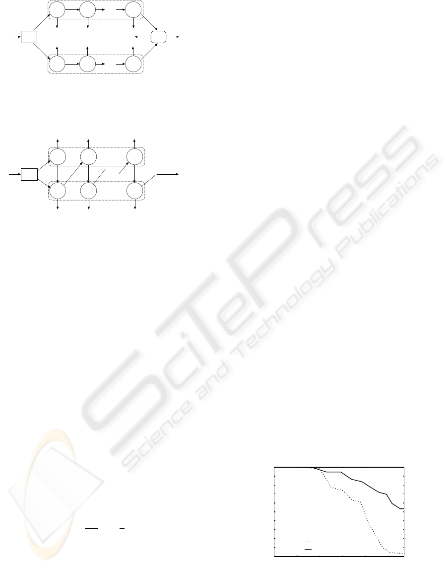
The result of our experiment is shown in Figure 7.
The horizontal axis shows false positive rate and the
vertical axis shows true positive rate. The horizontal
axis is a logarithmic axis to show the difference of the
graphs more clearly.
This graph shows that the precision of InfoBoost
is higher than that of AdaBoost. The true positive
rate of AdaBoost impatiently decreases when the false
positive rate is small. When the false positive rate is
small, there are less misclassified non-face samples
than misclassified face samples. InfoBoost can fo-
cus on both misclassified non-face and face samples
separately, thus InfoBoost can reduce false positive
rate with reduction of true positive rate. In contrast,
AdaBoost cannot focus on the misclassified non-face
samples and but can focus on the misclassified face
samples. That is because AdaBoost does not use the
true classes of samples and cannot discriminate be-
tween misclassified face samples and misclassified
non-face samples. AdaBoost cannot distinguish be-
tween misclassified faces and misclassified non-faces,
and cannot focus on misclassified non-faces, thus Ad-
aBoost reduce true positive rate without reduction of
false positive rate, and the precision of AdaBoost im-
patiently decreases.
0.5
0.55
0.6
0.65
0.7
0.75
0.8
0.85
0.9
0.95
1
1e-05 0.0001 0.001 0.01 0.1 1
AdaBoost
InfoBoost
True Positive Rate
False Positive Rate
Figure 7: Precision of Classifier.
Second, we perform the experiment of face track-
ing with 3D model, and examine the accuracy of
the classifier for each angle (-60, -30, 0, 30, 60 de-
VISAPP 2006 - IMAGE UNDERSTANDING
82

grees). The training set this time will consist of the
training, and the test sets will in the first experiment.
We use Head Pose Image Database of Pointing’04
(N. Gourier, 2004) as test set. This data set contain
multidirectional face images (vertical angle={-90, -
60, -30, -15, 0, +15, +30, +60, +90}, and horizontal
angle={-90, -75, -60, -45, -30, -15, 0, +15, +30, +45,
+60, +75, +90}). We use a part of these samples,
whose vertical angles are 0, and horizontal angles
are {-75, -60, -45, -30, -15, 0, +15, +30, +45, +60,
+75}. There are 30 sample images for each degree,
basically the maximum number of detected faces is
30. Besides, the number of evaluated sub-images is
about 4800000. Thus the maximum number of de-
tected negative samples is about 4800000.
We show two figures indicating the accuracy of
classifiers in Figure 8 and Figure 9. We represent
the classifier aiming at detecting faces rotated with
θ degrees as Classifier[θ], and samples rotated with
θ degrees as Samples[θ]. Most classifiers can detect
faces rotated with an angle close to that of the classi-
fier, and the number of mis-detected non-faces is not
many. For example, Classifier[0] classifies Sample[0]
correctly with high precision. However, there are two
exceptions.
One of them is that Classifier[−30] and
Classifier[+30] have the highest detection rate
on Samples[−15] and Samples[+15]. The reason of
angle mismatch is as follows: The structure of 3D
face model is too simple to represent human faces
correctly. Additionally, the test samples are taken by
only one camera, and faces are turned toward a sign
on the wall that indicates the direction. When the
samples were being taken, some people of the test
sample only focused their eyes on the sign instead of
rotating their heads, thus their face direction is not
turned toward the sign.
The other exception is that Classifier[−60] and
Classifier[+60] have the highest detection rate on
Samples[0]. For this case, we consider the reason is
self-occlusion of 3D model. If the angle is -60 or 60
degrees, self-occlusion of 3D model emerges and we
cannot use left or right half-face detectors. Accord-
ingly, the Classifier[−60] and the Classifier[+60] de-
tects half of the whole face, thus the number of de-
tected faces in Samples[0] is increased.
Third, we compare the detection speed between
the classifiers using the new cascading structure (Fig-
ure 5) and the classifiers using old one (Figure 6) on
all the samples used in the second experiment. If we
use the new cascading structure, we can detect faces
in an image whose size is 320x240 pixels, in about
0.036 seconds on 3.2GHz Pentium 4. If we do not
use the new cascading structure, the calculation time
is about 0.043 seconds. Hence, our new structure of
cascading is effective for reduction of time complex-
ity.
Figure 8: Number of Detected Faces for Each Direction.
Figure 9: Number of Detected Non-Faces for Each Direc-
tion.
Fourth, we execute the learning process with ran-
dom sampling, and evaluate it. We extracted train-
ing sets from the same data set, which is used as the
training set in the second experiment. The learning
time with random sampling is about 2.5 hours, and
that without random sampling is about 2 days. Ad-
ditionally, the result of face detection with random
sampling is shown in Table 1. The numbers of de-
tected faces and non-faces for each direction are re-
duced compared to the detection result without ran-
dom sampling. Accordingly, precision is reduced and
recall is improved. Total accuracy is not reduced. In
conclusion, random sampling reduces the time com-
plexity of learning without reducing the accuracy of
the face detector.
Table 1: Number of Detected Faces/Non-Faces for Each Di-
rection With Random Sampling.
-60 -30 0 +30 +60
-75 23 / 10 0 / 0 1 / 0 0 / 0 0 / 14
-60 17 / 6 0 / 0 2 / 0 0 / 0 0 / 9
-45 11 / 9 1 / 0 2 / 0 0 / 0 0 / 6
-30 9 / 10 7 / 0 12 / 1 0 / 0 1 / 3
-15 8 / 11 14 / 0 20 / 0 3 / 0 5 / 1
0 6 / 5 13 / 0 25 / 0 17 / 0 11 / 3
+15 3 / 2 2 / 0 14 / 1 17 / 1 15 / 1
+30 1 / 2 1 / 0 5 / 0 7 / 0 5 / 3
+45 0 / 10 0 / 0 0 / 1 5 / 0 6 / 2
+60 0 / 10 0 / 0 0 / 1 2 / 0 12 / 4
+75 0 / 7 0 / 0 0 / 0 0 / 0 11 / 8
Fifth, we increase the weight of misclassified face
samples in the learning process. The way we ex-
MULTIDIRECTIONAL FACE TRACKING WITH 3D FACE MODEL AND LEARNING HALF-FACE TEMPLATE
83

tracted training sets is the same as that in the fourth
experiment. After updating the weights of samples,
we double the weights of misclassified face samples.
The result of face detection is shown in Table 2.
Looking at the result of Classifier[−30], Classifier[0]
and Classifier[+30], we see the number of detected
faces is not increased and the number of detected non-
faces is decreased. The reason of this is that we use
parameters maxF P and minT P to repeat and finish
the learning process. These parameters are stronger
than modification of weights. Hence, the modifica-
tion of weights cannot increase the precision of face
detector. However, it can reduce its time complex-
ity, because the learning process focuses more on the
misclassified faces and converges faster. In this case,
we can detect faces in an image whose size is 320 by
240 pixels, in about 0.023 seconds on 3.2GHz Pen-
tium 4, which is faster than that without modifying
the weights.
Table 2: Number of Detected Faces/Non-Faces for Each Di-
rection With Random Sampling and biased InfoBoost.
-60 -30 0 +30 +60
-75 26 / 1 0 / 0 0 / 0 0 / 0 0 / 15
-60 22 / 2 0 / 0 0 / 0 0 / 0 0 / 10
-45 18 / 3 1 / 0 0 / 0 0 / 0 0 / 11
-30 13 / 8 1 / 0 4 / 0 0 / 0 9 / 2
-15 10 / 10 2 / 0 12 / 0 0 / 0 9 / 2
0 7 / 8 0 / 0 20 / 0 10 / 0 17 / 2
+15 3 / 6 1 / 0 9 / 0 8 / 0 14 / 9
+30 2 / 10 0 / 0 1 / 0 2 / 0 11 / 5
+45 0 / 10 0 / 0 0 / 0 0 / 0 12 / 8
+60 0 / 14 0 / 0 0 / 0 1 / 0 17 / 2
+75 0 / 11 0 / 0 0 / 0 0 / 0 18 / 5
7 CONCLUSIONS AND FUTURE
WORK
In this paper, we tried to improve the precision of a
classifier by using InfoBoost algorithm and tried to
detect not only frontal faces but also side faces by us-
ing 3D model and half-face templates. Additionally
we extend the classifier cascade, and reduce the time
complexity of learning and face detection.
However, we cannot detect faces rotated around the
horizontal axis, or the axis vertical to the image. If we
rotate the 3D model around these axes and project the
features from 3D model to 2D space, these Haar-Like
feature rectangles are deformed. In our algorithm, we
can only calculate upright rectangles. Thus, we must
think about a fast algorithm to calculate these feature
values.
Furthermore, with the extensions in this paper, the
time complexity of face detection is increased. We
must reduce the time complexity by reducing the
images evaluated with face detector or some other
method. In the process of extracting sub-images
from the target image, if we use skin colors to de-
tect face candidate regions, the number of evaluated
sub-images are reduced. Therefore, the precision of
classifier may be improved and time complexity may
be reduced.
Likewise, we must perform more experiments with
different training and test samples. When we perform
experiments with only one training set and one test
set, the result depends only on these samples. Conse-
quently, if these samples are not trusty, the experiment
result is not trusty either.
REFERENCES
Aslam, J. A. (2000). Improving Algorithms for Boosting.
In Proc. of 13th Annual Conference on Computational
Learning Theory (COLT 2000), pages 200–207.
Chernoff, H. (1952). A Measure of Asymptotic Efficiency
for Tests of a Hypothesis Based on the Sum of Obser-
vation. Ann. Math. Stat., 23:493–509.
Freund, Y. and Schapire, R. E. (1996). Experiments with
a New Boosting Algorithm. In Proc. of 13th Interna-
tional Conference on Machine Learning (ICML’96),
pages 148–156.
Georghiades, A., Belhumeur, P., and Kriegman, D. (2001).
From Few to Many: Illumination Cone Models
for Face Recognition under Variable Lighting and
Pose. IEEE Trans. Pattern Anal. Mach. Intelligence,
23(6):643–660.
Gross, R., Matthews, I., and Baker, S. (2004). Constructing
and fitting Active Appearance Models with occlusion.
In Proc. of the IEEE Workshop on Face Processing in
Video (FPIV’04).
N. Gourier, D. Hall, J. L. C. (2004). Estimating Face Ori-
entation from Robust Detection of Salient Facial Fea-
tures. In Proc. of Pointing 2004, International Work-
shop on Visual Observation of Deictic Gestures.
Pradeep, P. P. and Whelan, P. F. (2002). Tracking of facial
features using deformable triangles. In Proc. of the
SPIE - Opto-Ireland 2002: Optical Metrology, Imag-
ing, and Machine Vision, volume 4877, pages 138–
143.
Ross, D. A., Lim, J., and Yang, M.-H. (2004). Adaptive
Probabilistic Visual Tracking with Incremental Sub-
space Update. In Proc. of Eighth European Confer-
ence on Computer Vision (ECCV 2004), volume 2,
pages 470–482.
Viola, P. and Jones, M. (2001). Rapid Object Detection us-
ing a Boosted Cascade of Simple Features. In Proc. of
IEEE Conf. on Computer Vision and Pattern Recogni-
tion, pages 511–518.
Zhu, Z. and Ji, Q. (2004). Real Time 3D Face Pose Tracking
From an Uncalibrated Camera. In Proc. of the IEEE
Workshop on Face Processing in Video (FPIV’04).
VISAPP 2006 - IMAGE UNDERSTANDING
84
