
A STATISTICAL BASED APPROACH FOR REMOVING HEAVY
TAIL NOISE FROM IMAGES
M. El Hassouni and H. Cherifi
LIRSA, University of Dijon
9, avenue Alain Savary 21000 Dijon, France
Keywords:
image restoration, l
p
-norm filter, α-stable processes, Fractional lower order statistics.
Abstract:
In this paper, we propose to use a class of filters based on fractional lower order statistics (FLOS) for still
image restoration in the presence of α-stable noise. For this purpose, we present a family of 2-D finite-
impulse response (FIR) adaptive filters optimized by the least mean l
p
-norm (LMP) algorithm. Experiments
performed on natural images prove that the proposed algorithms provide superior performance in impulsive
noise environments compared to LMS and Weighted Myriad filters.
1 INTRODUCTION
Several distributions that exist can be good candi-
dates for modelling noise signals. The most common
in the literature, and especially in signal and image
processing, is the Gaussian distribution. The use of
the Gaussian distribution is frequently motivated by
the physics of the problem, and in most cases it en-
sures an analytical solution. This has led to the de-
velopment of numerous algorithms based on second-
order statistics.
However, in many real-world problems the noise
encountered is more impulsive in nature than that pre-
sented by a Gaussian distribution. Important non-
Gaussian impulsive noise, found in radar and mobile
communications for example, can be efficiently mod-
elled by infinite variance processes for which the the-
ory of SOS is not useful(Gonzales and Arce, 1997).
There exists a class of distributions, called α-stable
distributions that can be used to model these types
of noise. A variety of FLOS-based algorithms have
been proposed to filter α-stable random processes
(Aydin et al., 1999; Shao and Nikias, 1993; Kid-
mose, 2000). This property has been used exten-
sively in one-dimensional (1-D) signal processing,
e.g. in removing some undesired effects in commu-
nication channels or synthesizing a deconvolution fil-
ter. Nonlinear least l
p
-norm polynomial filters ex-
pansion is a powerful tool in signal processing (Ku-
ruoglu et al., 1998; Kuruoglu, 2002). However, a
serious problem is the increased filter complexity as
compared to linear filtering. Developing this tech-
niques for two-dimensional (2-D) signal processing
(i.e. image processing) is of current research inter-
est. Weighted myriad filters (WMyF) have been used
with considerable success in robust communications
and image processing. They have been derived based
on the Cauchy distribution, which is a special case
of α-stable distributions. WMyF are inherently more
powerful than weighted median filters (WMF), which
along with other order statistics filters, have been used
widely in image processing, due to their edge preser-
vation and outlier rejection properties (Gonzalez and
Arce, 1996).
In this paper, we present a 2-D adaptive least l
p
-
norm (LMP) filter and its normalized version for im-
age restoration under additive α-stable noise. The al-
gorithms are based on fractional lower order statis-
tics (FLOS). The performances of these algorithms
are compared to those of the normalized least mean
square-type algorithm which is developed under the
Gaussian assumption.
The organization of the article is as follows. In
Section 2, we present the problem formulation with
some definitions of the α-stable processes. Section 3
is then devoted to the presentation of the 2-D adaptive
l
p
-norm filter and some related work. Finally, experi-
mental results and some concluding remarks are given
in Section 4 and Section 5, respectively.
157
El Hassouni M. and Cherifi H. (2006).
A STATISTICAL BASED APPROACH FOR REMOVING HEAVY TAIL NOISE FROM IMAGES.
In Proceedings of the First International Conference on Computer Vision Theory and Applications, pages 157-161
DOI: 10.5220/0001371901570161
Copyright
c
SciTePress

2 PROBLEM FORMULATION
Let us consider that the observed image g(i, j) can be
expressed as a sum of noise-free image f(i, j) plus
(2-D) additive noise, i.e.,
g(i, j)=f(i, j)+η(i, j) (1)
where (i, j) denotes the pixel coordinates. In im-
age processing a neighborhood is defined around each
pixel (i, j). The random noise η(i, j) is modelled as
a symmetric α-stable process (SαS).
The stable distribution law is a direct generalization
of the Gaussian distribution and in fact includes the
Gaussian as a limiting case. The main difference be-
tween the non-Gaussian stable distribution and the
Gaussian distribution is that the tails of the stable
density are heavier than those of the Gaussian den-
sity. The characteristic of the stable distribution is
one of the main reasons why the stable distribution is
suitable for modeling signals and noise of impulsive
nature. The α-stable distributions do not have close
form probability density function except the cases
α =1(Cauchy distribution) and α =2(Gaussian
distribution). The SαS probability density function
(pdf) is defined by means of its characteristic function
φ(ω)=exp(δiω − γ|ω|
α
) (2)
where
• i) α(0 <α≤ 2) is the characteristic exponent,
controlling the heaviness of the pdf tails,
• ii) γ(γ>0) is the dispersion, which plays an anal-
ogous role to the variance, and
• iii) δ is the location parameter, the symmetry axis
of the pdf.
Due to the heavy tails, stable distributions do not have
finite second- or higher-order moments, except the
limiting case of α =2. More precisely, for X,an
α-stable random variable with (0 <α<2)
E[|X|
p
]=∞ if p ≥ α (3)
However, for 0 <p≤ α, the fractional lower order
moment (FLOM) is finite, i.e.,
E[|X|
p
] < ∞ if 0 ≤ p<α (4)
If α =2, then
E[|X|
p
] < ∞ for p ≥ 0 (5)
The fractional pth-order moment of an SαS random
variable with zero location parameter, δ =0,isgiven
by
E[|X|
p
]=C(p, α)γ
p/α
, for 0 <p<α
(6)
where
C(p, α)=
2
p+1
Γ(
p+1
2
)Γ(−p/α)
α
√
πΓ(−p/2)
(7)
Γ(.) denotes the gamma function.
3 2-D ADAPTIVE LEAST
L
P
-NORM FILTER
Our purpose is to design a filter on the pixel neigh-
borhood (called the filter window) that aims at es-
timating the noise-free central image pixel value by
minimizing a certain criterion. Among the several fil-
ter masks that are used in digital image processing,
we rely on the square window of dimension Ξ × Ξ
where Ξ is generally assumed to be an odd number,
i.e., Ξ=2ξ +1.
g(i − ξ, j − ξ) g(i − ξ, j − ξ +1) ... g(i − ξ, j + ξ)
::
g(i + ξ, j − ξ) g(i + ξ, j − ξ +1) ... g(i + ξ, j + ξ)
(8)
Let us rearrange the above Ξ × Ξ filter window in
a lexicographic order (i.e., row by row) to a N × 1
vector, where N =Ξ
2
.
We assume that the filter window is sliding over im-
age in a raster scan fashion. If K and L denote the
image rows and columns respectively, a scalar run-
ning index m is defined by
m =(i−1)K+j 1 ≤ i ≤ K 1 ≤ j ≤ L
(9)
Consider an adaptive 2D FIR filter, the intensity esti-
mate at pixel (i, j) is given by :
ˆ
f(i, j)=
+ξ
k=−ξ
+ξ
l=−ξ
a(k, l)g(i − k, j − l) (10)
Where
ˆ
f(i, j) is the filtered gray-level pixel located at
(i, j); a(k, l) is the filter weights around pixel (i, j);
g(i − k, j − l) is the corrupted pixel at location (i −
k, j − l).
The filter weights are estimated by minimizing a cost
function J(e(i, j)), where e(i, j)=
ˆ
f(i, j) − f(i, j)
is the filter estimation error at pixel (i, j).
The update equations are defined by :
ˆa
m+1
(k, l)=ˆa
m
(k, l)+µ
∂J(e(i, j))
∂a
m
(k, l)
(11)
Where µ is the step-size parameter that controls the
stability and the rate of convergence.
3.1 Related Work
The classical and the simplest adaptive type algorithm
is the least mean square (LMS). LMS adapts the lin-
ear filter weights with every coming sample in the
steepest descent direction. The cost function can be
defined as :
J(e(i, j)) = E{e
2
(i, j)} (12)
the update equations of LMS filter and it’s adaptive
version NLMS filter are defined by:
VISAPP 2006 - IMAGE FORMATION AND PROCESSING
158

• 2-D LMS:
ˆa
m+1
(k, l)=ˆa
m
(k, l)+2µe(i, j)g(i − k, j − l)
• 2-D NLMS:
ˆa
m+1
(k, l)=ˆa
m
(k, l)+2µ
e(i,j)
g(i,j)
2
+λ
g(i −k, j −
l)
Where λ is an algorithm parameter, the quantity
g(i, j)
2
is given by:
g(i, j)
2
=
+ξ
k=−ξ
+ξ
l=−ξ
|g(i − k, j − l)|
2
(13)
3.2 Proposed 2-D Adaptive Least l
p
Norm Filter
The LMS algorithm has sever convergence problems
for signals with more probability mass in the tails,
than the Gaussian distribution. Recently filter theory
for SαS signals has been developed, and the least
Mean p-norm (LMP) algorithm has been proposed
(Shao and Nikias, 1993). The objective is to mini-
mize the dispersion of the error (p-norm cost func-
tion) which is defined by :
J(e(i, j)) = E{|e(i, j)|
p
} (14)
So, the update equation is:
• 2-D LMP :
ˆa
m+1
(k, l)=ˆa
m
(k, l)+
µp|e(i, j)|
p−1
sign(e(i, j))g(i − k, j − l)
Although LMP is much more robust to impulsive
noise than LMS, in some cases with the appearance
of extremely impulsive noise it can become unsta-
ble. Motivated by the stability and increased speed
of the normalized version of LMS, namely NLMS, an
adaptive version for LMP, namely normalized LMP
(NLMP), which can be expressed by :
• 2-D NLMP :
ˆa
m+1
(k, l)=ˆa
m
(k, l)+
µp
|e(i,j)|
p−1
sign(e(i,j))
g(i,j)
p
p
+λ
g(i − k, j − l)
Where is a small λ which is included to avoid the di-
vision by zero, the quantity g(i, j)
p
p
is given by:
g(i, j)
p
p
=
+ξ
k=−ξ
+ξ
l=−ξ
|g(i − k, j − l)|
p
(15)
In all of these algorithms, the coefficient vector can be
conveniently initialized to a good guess or to a zero
vector if no prior information is available.
4 EXPERIMENTAL RESULTS
Here we present a simulation example of our appli-
cation experiments demonstrating the behavior of the
2-D adaptive lp-norm filter. Due to the lack of origi-
nal noise-free images in practice, the filters are trained
over an image other than those to be filtered in or-
der to represent a realistic scenario. Specially, the
couple image is used in deriving the weighting co-
efficients, which are then used in filtering other im-
ages (Kotropoulos and Pitas, 2001). The images are
corrupted by symmetrical α-stable noise with (α =
0.5; ...;1.5), (γ =1) and (δ =0).
For objective quality evaluation, two criteria have
been employed, namely, the fractional order SNR
(FSNR(Kuruoglu et al., 1998)) defined as the loga-
rithm of the ratio of the pth-order moments of the
noise and the signal where 0 <p<αinstead of
their powers, that is,
FSNR(dB) = 10 log
10
K
i=1
L
j=1
|f(i, j)|
p
K
i=1
L
j=1
|
ˆ
f(i, j) − f (i, j)|
p
(16)
This evaluation criterion may favor the least l
p
-
norm filters since it is defined for the pth-order. How-
ever, we propose to use the Mean Structural SIMilar-
ity (MSSIM) index described in (Wang et al., 2004).
MSSIM(X, Y )=
1
M
M
j=1
SSIM(x
j
,y
j
) (17)
where X and Y are the reference and the distorted
image, respectively; x
j
and y
j
are the image contents
at the jth local window; and M is the number of local
windows of the image. The SSIM index is defined by:
SSIM(x, y)=
(2µ
x
µ
y
+ C1)(2σ
xy
+ C2)
(µ
2
x
+ µ
2
y
+ C1)(σ
2
x
+ σ
2
y
+ C2)
(18)
Where the constants C1=(K
1
L
2
) and C2=
(K
2
L
2
) are included to avoid the instability when
µ
2
x
+ µ
2
y
and σ
2
x
+ σ
2
y
are very close to zero, respec-
tively. L is the dynamic range of the pixel values (255
for 8-bit grayscale images), and K
1
, K
2
are small
constants 1.
A point that needs some clarification is the choice
of the scale of the p norm where the performance
comparisons have to be made. So, the common way
of determining p of the algorithm is to use the equal-
ity suggested by Money and al. (Money et al., 1982)
that relates the kurtosis of the non-Gaussian data p of
the l
p
-norm minimization algorithm, which is
p =
9
K
2
+1 (19)
where K is the kurtosis measure. Although this mea-
sure is very commonly used in literature, we have
doubts concerning its efficiency, since the kurtosis
is defined through the fourth and the second order
moments which are not finite for α-stable distributed
random variables. In our simulations, the p values
A STATISTICAL BASED APPROACH FOR REMOVING HEAVY TAIL NOISE FROM IMAGES
159

have been tuned experimentally, Figure 1 shows an
example of PSNR and MSSIM values obtained sev-
eral values of p. It is shown that both measures give
the similar optimum values of p. For example, with
α =1.5 the optimum value of p is around 1.3, and
with α =1.9 the optimum value of p is around 1.7.
We show in Figure 2 the results of the adaptive l
p
-
norm filter in suppressing impulsive noise in Lena im-
age. Figure 2(a) shows the image corrupted by im-
pulsive noise which is represented by Symmetrical α-
stable noise (α=0.5). The output of the NLMS filter
is shown is Figure 2(b). Figure 2(c) shows the filtered
image by using the weighted median filter (WMF).
The filtered image using the weighted myriad filter
(WMyF) is shown in Figure 2(d). Figure 2(e) shows
the filtered image using the 2-D adaptive LMP filter
with fixed step-size. Finally, the filtered image by the
normalized l
p
-norm filter is shown in Figure 2(f). The
filter parameters have been tuned to obtain the best vi-
sual results.
The visual quality demonstrates the superiority of
using fractional lower-order statistics filtering algo-
rithms which gives a good performance with edges
and fine image details preserving.
Table 1 summarizes respectively the FSNR and
the MSSIM achieved by the adaptive proposed fil-
ters with different values of α . According to
these results, the filtered image using l
p
-norm fil-
ter has higher FSNR and MSSIM improvement from
the LMP/NLMP linear equalizers than those of the
NLMS filter, weighted median filter and weighted
myriad filter. The measures achieved by the normal-
ized l
p
-norm filter give good improvement in term of
visual quality and signal-to-noise ratio improvement.
When a reference image is not available. We use
the same methodology as described in (Kotropoulos
and Pitas, 2001). We have tested the robustness of
the filter coefficients that are determined at the end
of a training session and are applied to filter a noisy
image that has been produced by corrupting a differ-
ent reference image than the one used in the training
session. In Figure 3, we present a filtered house im-
age using the coefficients determined at the end of a
training session on lenna image. The same noise pa-
rameters have been used during the training session.
When, regarding the quality of the filtered images and
the quality evaluation measures, we can say that the
proposed filter is very good for α-stable noise perfor-
mance measurement.
5 CONCLUSION
In this paper, we presented a 2-D adaptive l
p
-norm
filter for noise suppression in images. Experimental
results on natural images showed marked improve-
ment in visual and numerical qualities when using the
normalized l
p
-norm algorithm adaptation. The filter
is very suitable for α-stable and impulsive noise re-
moval.
REFERENCES
G. Aydin, O. Arikan, and E. Cetin. Robust adaptive filter-
ing algorithms for α-stable random processes. IEEE
Trans. On Circuits and Systems II, vol. 46, N. 2, pp.
198-202, February 1999.
M. Shao, C. L. Nikias. Signal processing with fractionnal
lower order moments : Stable processes and their ap-
plications. Proc. IEEE, vol. 81, pp. 986-1009, 1993.
J. G. Gonzalez, G. R. Arce. Weighted myriad filters :
A robust filtering framework derived from alpha-
stable distributions. Proc. of the IEEE Int. Conf. on
Acoustics, Speech and Signal Processing, Atlanta,
GA, May 1996, Vol. 5, pp. 2833-2836.
J. G. Gonzales, G.R. Arce. Zero-order statistics : a signal
processing framework for very impulsive processes.
Proceedings of the IEEE Signal Processing Workshop
on Higher-Order Statistics, Banff, Canada, July 1997,
pp. 254-258.
P. Kidmose. Adaptive filtering for non-Gaussian noise
processes. Proceedings of International Confer-
ence on Acoustics, Speech and Signal Processing,
ICASSP2000, pp. 424-427.
Ercan E. Kuruoglu, Peter J. W. Rayner, William J. Fitzger-
ald. Least l
p
-norm impulsive noise cancellation with
polynomial filters. Signal Processing. v. 69, pp. 1-14.
1998.
A. Ben Hamza and H. Krim. Image denoising : A nonlin-
ear robust statistical approach. IEEE Trans. on Signal
Processing, Vol. 49, N0. 12, Decembre 2001.
Ercan E. Kuruoglu. Nonlinear least lp-norm filters for non-
linear autoregressive α-stable processes. Digital Sig-
nal Processing 12, 119-142 (2002).
O. Tanrikulu and A. G. Constantindes, ”Least-mean Kur-
tosis : A novel higher-order statistics based adaptive
filtering algorithm”, Electronics Letters, vol. 30, no.
3, pp. 189-190, February 1994.
C. Kotropoulos and I. Pitas, Nonlinear Model-Based Im-
age/Video Processing and Analysis, J. Wiley, 2001.
A. H. Money, J. F. Affleck-Graves, G.D.I. Barr, The linear
regression model: L-p-norm estimation and the choice
of p, Communications in Statist. Simulation Comput.
11 (1) (1982) 89-109.
Zhou Wang, Alan C. Bovik, Hamid R. Sheikh and Eero
P. Simoncelli. Image quality assessment: from er-
ror measurement to structural similarity. To appear in
IEEE transactions on image processing, vol. 13, No.
1, January 2004.
VISAPP 2006 - IMAGE FORMATION AND PROCESSING
160
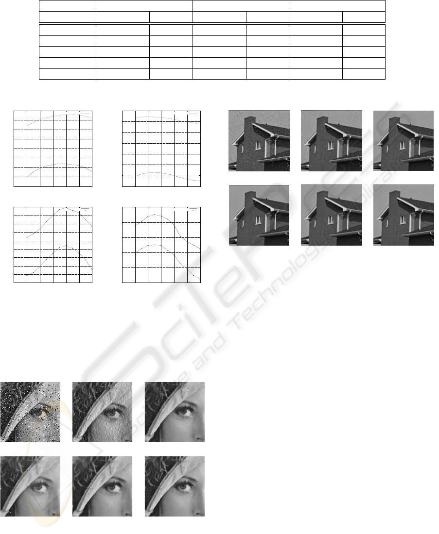
Table 1: FSNR and MSSIM achieved by different filters.
Alpha values α=0.5 α=1.0 α=1.5
Measure FSNR(dB) MSSIM FSNR(dB) MSSIM FSNR(dB) MSSIM
2-D NLMS 11.46 0.4865 14.01 0.806 13.66 0.824
2-D WMF 15.74 0.8230 15.35 0.8592 13.97 0.8678
2-D WMyF 15.87 0.8422 16.53 0.927 14.63 0.9034
2-D LMP 16.85 0.8736 16.28 0.9064 15.32 0.9126
2-D NLMP 17.30 0.8984 16.33 0.9162 15.55 0.9135
33.8
34
34.2
34.4
34.6
34.8
35
35.2
35.4
0.8 1 1.2 1.4 1.6 1.8 2
PSNR(dB)
p
’LMP_1.9’
’NLMP_1.9’
31
31.2
31.4
31.6
31.8
32
32.2
32.4
0.8 1 1.2 1.4 1.6 1.8 2
PSNR(dB)
p
’LMP_1.5’
’NLMP_1.5’
(a) (b)
91.8
92
92.2
92.4
92.6
92.8
93
93.2
93.4
93.6
0.8 1 1.2 1.4 1.6 1.8 2
MSSIM
p
’nlmp_1.9’
’lmp_1.9’
90
90.5
91
91.5
92
92.5
0.8 1 1.2 1.4 1.6 1.8 2
MSSIM
p
’nlmp_1.5’
’lmp_1.5’
(c) (d)
Figure 1: a) PSNR versus p for Lenna corrupted with SαS
α =1.9. b) PSNR versus Lenna corrupted with SαS α =
1.5. c) MSSIM versus p for Lenna corrupted with SαS
α =1.9. d) MSSIM versus Lenna corrupted with SαS
α =1.5.
(a) (b) (c)
(d) (e) (f)
Figure 2: (a) Corrupted Lenna image (α =0.5) (b) Fil-
tered image using NLMS filter (c) Weighted Median Filter
(d) Filtered image using weighted myriad filter (e) filtered
image using LMP filter (f) filtered image using NLMP filter.
(a) (b) (c)
(d) (e) (f)
Figure 3: (a) Corrupted house image (α =0.9)
(b) Filtered image using NLMS filter (FSNR=12.49 dB,
MSSIM=0.74) (c) Weighted Median Filter (FSNR=13.94
dB, MSSIM=0.82) (d) Filtered image using weighted myr-
iad filter (FSNR=15.50 dB, MSSIM=0.87) (e) filtered im-
age using LMP filter (FSNR=14.84 dB, MSSIM=0.86)
(f) filtered image using NLMP filter (FSNR=16.33 dB,
MSSIM=0.92.)
A STATISTICAL BASED APPROACH FOR REMOVING HEAVY TAIL NOISE FROM IMAGES
161
