
JOINT PRIOR MODELS OF MUMFORD-SHAH REGULARIZATION
FOR BLUR IDENTIFICATION AND SEGMENTATION IN VIDEO
SEQUENCES
Hongwei Zheng and Olaf Hellwich
Computer Vision & Remote Sensing, Berlin University of Technology
Franklinstrasse 28/29, Sekretariat FR 3-1, D-10587 Berlin
Keywords:
Bayesian estimation, point spread function, blind image deconvolution, Mumford-Shah functional, partial
differential equations, Γ-convergence, piecewise smooth approximate, graph-grouping, segmentation.
Abstract:
We study a regularized Mumford-Shah functional in the context of joint prior models for blur identification,
blind image deconvolution and segmentation. For the ill-posed regularization problem, it is hard to find a
good initial value for ensuring the soundness of the convergent value. A newly introduced prior solution
space of point spread functions in a double regularized Bayesian estimation can satisfy such demands. The
Mumford-Shah functional is formulated using Γ-convergence approximation and is minimized by projecting
iterations onto an alternating minimization within Neumann conditions. The pre-estimated priors support the
Mumford-Shah functional to decrease of the complexity of computation and improve the restoration results
simultaneously. Moreover, segmentation of blurred objects is more difficult. A graph-theoretic approach is
used to group edges which driven from the Mumford-Shah functional. Blurred objects with lower gradients
and objects with stronger gradients are grouped separately. Numerical experiments show that the proposed
algorithm is robust and efficiency in that it can handle images that are formed in different environments with
different types and amounts of blur and noise.
1 INTRODUCTION
The challenge of blind image deconvolution (BID) is
to uniquely define the optimized signals only from
the degraded images. Segmentation of blur degraded
images becomes more important. An ideal image f
in the object plane is degraded by a linear space-
invariant point spread function (PSF) h with an ad-
ditive Gaussian white noise n using the linear degra-
dation model g = hf + n. An observed image in the
image plane g is formed by two unknown conditions h
and n. The two-dimensional convolution is expressed
as hf = Hf = Fh, where H and F are block-
Toeplitz matrices and can be approximated by block-
circulant matrices for large images. The point spread
function (PSF) of blur is normally neither known nor
perfectly known. Such blur identification can be con-
sidered as blind image deconvolution.
A regularization theory (Tikhonov and Arsenin,
1977) presents numerous challenges as well as op-
portunities for further statistical and mathematical vi-
sion modeling to solve ill-posed problems. This for-
malism has been recognized as a unified framework
for studying several problems in early vision (Pog-
gio et al., 1985). However, the iterative Tikhonov
regularization (Katsaggelos et al., 1991) and the total
variation based regularization (Rudin et al., 1992) are
mostly focused on the image restoration, denoising,
or enhancement. A general regularization method
proposed by Mumford and Shah (Mumford and Shah,
1989) has some natural advantages not only in image
restoration but also in image segmentation. This func-
tional has formulated restoration and segmentation
problem mathematically in a energy minimization ap-
proach. Recently, the Mumford-Shah (MS) functional
has been extensively explored for image segmenta-
tion and restoration (Aubert and Kornprobst, 2002).
Through the literature study, most of these Mumford-
Shah based methods are intensively tested on the in-
fluences of noises or occlusions but less experiments
on the influences of blur. Blind image restoration and
segmentation of degraded images are difficult but be-
come more important in many vision systems. Com-
bination of blur identification, image restoration and
segmentation in the Mumford-Shah functional is a
reasonable strategy for such tasks due to the mutual
support of restoration and segmentation within a vari-
ational regularization. The reason is that accurate blur
56
Zheng H. and Hellwich O. (2006).
JOINT PRIOR MODELS OF MUMFORD-SHAH REGULARIZATION FOR BLUR IDENTIFICATION AND SEGMENTATION IN VIDEO SEQUENCES.
In Proceedings of the First International Conference on Computer Vision Theory and Applications, pages 56-63
DOI: 10.5220/0001371400560063
Copyright
c
SciTePress

identification and non-oversmoothing image restora-
tion preserve more discontinuities and edges for ac-
complishing successful image segmentation. Fur-
thermore, a variational regularization method expects
to find the optimal solution efficiently and robustly
based on some accurate prior information (Chan and
Wong, 2000). The effective prior information and
constraints are important to yield a unique solution
to the corresponding optimization procedure.
The Bayesian estimation framework provides a
structured way to include prior knowledge concerning
the quantities to be estimated. The Bayesian approach
is, in fact, the framework in which the most recent
restoration methods have been introduced. Studies on
existence, uniqueness, and stability of ill-posed early
vision problems and related problems are investigated
by Bertero, Poggio, and Torre (Bertero et al., 1988).
Blake et al. (Blake and Zisserman, 1987) proposed
the use of gradually non-convexity method, which can
be extended to the blurring problem. Molina and Rip-
ley (Molina and Ripley, 1989) proposed the use of a
log-scale for the image model. Green (Green, 1990)
and Bouman et al. (Bouman and Sauer, 1993) used
convex potentials in order to ensure uniqueness of the
solution. Recently, an appreciable extension of the
range of hyperparameter estimation methods is used
in Bayesian estimation. Molina et al. (Molina et al.,
1999) used a hierarchical Bayesian paradigm result-
ing from the set theoretic regularization approach for
estimating hyper-parameters. They also report that
the accuracy of the obtained statistic estimates for the
PSF and the image could vary significantly, depend-
ing on the initialization. To obtain accurate restora-
tions in the Bayesian approach, accurate prior knowl-
edge of PSF or image must be available.
In this paper, we investigate the Mumford-Shah
regularization for image segmentation and restoration
based on estimated PSF models. A newly introduced
solution space of PSF priors supports accurate para-
metric PSF in the form of Bayesian MAP estimation.
The PSF is estimated in a double L
2
norm regularized
Bayesian estimation framework and is used to support
the PSF value to the extended MS regularization. This
makes some important effects: Firstly, it becomes
possible to get good initial PSF value in Mumford-
Shah regularization via a statistic method to decrease
the complexity of computation. Secondly, it shows a
theoretically sound way of how Mumford-Shah reg-
ularization can be processed for segmentation and
restoration mutually. A graph cuts method is inte-
grated to the Mumford-Shah functional for partition-
ing and grouping edges driven from the Mumford-
Shah regularization. These edges are grouped using
different strengths of gradients. The experimental re-
sults shows that this method yields encouraging re-
sults and is robust under different kinds and amounts
of blur.
The paper is organized as follows. In Sect. (2),
Bayesian estimation in the context of double reg-
ularizations for blur identification is described. In
Sect. (3), the estimated PSFs support initial values for
the Mumford-Shah regularization. A graph-theoretic
concept is used to generate the result of segmentation.
Experimental results are shown in Sect. (4). Conclu-
sions are summarized in Sect. (5).
2 DOUBLE REGULARIZED
BAYESIAN ESTIMATION
2.1 Bayesian Estimation with Joint
Prior Solution Space of PSFs
The Bayesian MAP estimation utilizes a prior infor-
mation to achieve a convergent posterior. Following
a Bayesian paradigm, the true f, the PSF h and the
observed g are formulated in
p(f,h|g)=
p(g|f,h)p(f,h)
p(g)
∝ p(g|f,h)p(f,h) (1)
Applying the Bayesian paradigm to the blind decon-
volution problem, we try to get convergence values
from Eq. (1) with respect to f and h. This Bayesian
MAP approach can also be seen as a regularization
approach which combines optimization method for
minimizing two proposed cost functions in the image
domain and the PSF domain. The cost function of
the restored true image f and PSF h from Eq. (1) are
deducted respectively as the following,
L(f
(g,h)
) ∝ p(g|f,h)p(f)
L(h
(g,f)
) ∝ p(g|f,h)p
Θ
(h)
(2)
For the application of these equations, some con-
straints of the PSF and the image are assumed due to
the fact that the image pixels are independent identi-
cally distributed and does not influence the pixel cor-
relations.
The proposed prior solution space supports the
parametric structured PSFs in Bayesian estimation.
We define a set Θ as a solution space of Bayesian
estimation which consists of primary parametric blur
models as Θ={h
i
(θ),i =1, 2, 3, ..., N} and pre-
sented in Fig.(1). h
i
(θ) represents the ith paramet-
ric model of the PSF with its defining parameters θ
which denotes parameters of different PSFs in differ-
ent manifolds, and N is the number of blur kernels.
h
i
(θ)=
⎧
⎪
⎪
⎪
⎪
⎨
⎪
⎪
⎪
⎪
⎩
h
1
(θ) ∝ h(x, y; L
i
,L
j
)=1/K,
if |i|≤L
i
and |j|≤L
j
h
2
(θ) ∝ h(x, y)=K exp(−
x
2
+y
2
2σ
2
)
h
3
(θ) ∝ h (x, y, d, φ)=1/d,
if
x
2
+ y
2
≤ D/2, tan φ = y/x
JOINT PRIOR MODELS OF MUMFORD-SHAH REGULARIZATION FOR BLUR IDENTIFICATION AND
SEGMENTATION IN VIDEO SEQUENCES
57

ab
cd
Figure 1: PSFs in the prior solution space. (a) Original syn-
thetic image. (b) Pillbox PSF. (c) Gaussian PSF. (d) Linear
motion PSF.
h
1
(θ) is a Pillbox blur kernel with a length of radius
K. h
2
(θ) is a Gaussian PSF and can be characterized
by parameters with its variance σ
2
and a normalized
constant K. h
3
(θ) is a simple linear motion blur PSF
with a camera direction motion d and a motion an-
gle φ. The other blur structures like out-of-focus and
uniform 2D blur (Kundur and Hatzinakos, 1996) are
also built in the solution space as a priori informa-
tion. The prior solution space is constructed by a set
of parametric PSFs for estimating unknown PSFs in
the Bayesian MAP Estimation.
2.2 Estimation in the Image Domain
and the PSF Domain
Based on the Tikhonov regularization, Lagendijk et
al. (Lagendijk et al., 1988) made an extension of it by
means of the theory of projections onto convex sets
(POCS) (Katsaggelos et al., 1991) and the concepts
of norms in a weighted Hilbert space. A weighted
space-adaptive regularization equation then seeks to
minimize the following cost function
1
2
x∈Ω
w
1
(h(x) ∗ f (x) − g(x))
2
(3)
+
1
2
λ
x∈Ω
w
2
(c(x) ∗ f (x))
2
= min
where the cost function is minimized based on the
degraded image g(x), the ideal image f(x), and the
PSF h(x). c(x) is a regularization operator. x ∈ Ω,
Ω ⊂ R
2
is the support size of a given image. λ is
a regularization parameter that controls the trade-off
between the fidelity to the observation and smooth-
ness of the restored image. Weights w
1
and w
2
reduce
these two effects adaptively to achieve better visual
evaluation.
In the image domain, the cost function of image
estimate can be minimized iteratively in the weighted
space-adaptive regularized formulation. In this equa-
tion, p(g|f,h) follows a Gaussian distribution and
p(f) is a prior knowledge with some constraint con-
ditions.
L(f
(g,h)
) = arg max
f
[p(g|f,h)p(f)] (4)
=
1
2
x∈Ω
w
1
(g(x) − h(x) ∗ f(x))
2
+
1
2
λ
x∈Ω
w
2
(c
1
(x) ∗ f (x))
2
where p(f ) ∝ exp
−
1
2
λ
x∈Ω
w
2
(c
1
(x) ∗ f (x))
2
,
p(
g
f,h
) ∝ exp
−
1
2
x∈Ω
w
1
(g(x) − h(x) ∗ f(x))
2
.
Direct minimization of the cost function would lead
to excessive noise magnification due to the ill con-
ditioning of blur operator. A smoothness constraint
c
1
(x) is a regularization operator and is usually a
high-pass filter.
In the PSF domain, PSF can be seen as maximiz-
ing the conditional probability. However, manipula-
tion of probability density functions (PDF) of PSFs
in Bayesian estimation is difficult. A decision must
be made firstly to attribute an accurate initial value in
the regularization. The proposed prior solution space
supports the parametric structured PSFs in Bayesian
estimation. One more cost constraint of probability
for the estimated PSF is then added in the equation.
A new cost function for PSFs is following:
L(h
(g,f)
) = arg max
h
{p (g |h, f ) p
Θ
(h)}
=
1
2
x∈Ω
w
1
(g(x) − h(x) ∗ f(x))
2
+
1
2
β
x∈Ω
w
3
(c
2
(x) ∗ h(x))
2
+
1
2
γ
x∈Ω
w
4
|h − h
f
|
2
} (5)
Where p
Θ
(h) ∝
1
2
β
x∈Ω
w
3
(c
2
(x) ∗ h(x))
2
+
1
2
γw
4
|h − h
f
|
2
is the prior knowledge and need to
be computed firstly. h is a current estimated PSF and
h
f
is the final result of the estimated PSF for a given
image. Since both ideal and observed image repre-
sent intensity distributions that cannot take negative
values, the PSF coefficients are always nonnegative,
h(x) ≥ 0. Furthermore, since the image formation
system normally does not absorb or generate energy,
the PSF should satisfy
x∈Ω
h(x) = 1.0. The prob-
ability of current PSF is computed in a Gaussian den-
sity function:
h
i
(θ
∗
) = arg max
θ
p (h
i
(θ) |h)
= arg max
θ
log
(2π)
−
L∗B
2
dd
−
1
2
∗ exp
−
1
2
(h
i
(θ) − h)
T
−1
dd
(h
i
(θ) − h)
VISAPP 2006 - IMAGE FORMATION AND PROCESSING
58
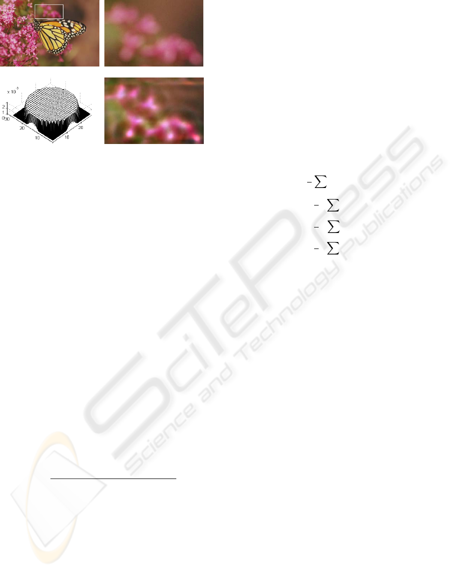
(a) standard test image (b) cropped blur part
(c) estimated PSF via Bayesian (d) restored using estimated PSF
Figure 2: A estimated PSF using the prior solution space in
the Bayesian MAP Framework.
We define the likelihood of the neighbor h and in re-
sembling the ith parametric model h
i
(θ), h
i
(θ) ∈ Θ.
The first subscript i denotes the index of the blur
kernel. The modeling error d = h
i
(θ) − h is as-
sumed to be a zero-mean homogeneous Gaussian dis-
tributed white noise process with covariance matrix
dd
= σ
2
d
I independent of f (x, y). L ∗ B is an
assumed support size of the blur kernel. The like-
lihood of the current PSF l
ij
(h) is computed using
an Euclidean distance between the current PSF h and
the corresponding probability model h
i
(θ
∗
), l
ij
(h)=
N
i=1
exp{−|h
i
(θ
∗
) − h|
2
/[2tr(
dd
)]}.
Motivated by the K-nearest neighbor concept, a
weighted mean filter is used to determine the likeli-
hood of h belonging to the ith parametric blur model.
The mean value of likelihood l
m
(h) is l
ij
(h) weight-
divided by d(h, h
j
). d(h, h
j
) is the Euclidean dis-
tance between h and its neighbor h
j
. The weighted
mean likelihood l
m
(h) should depend on two condi-
tions. The first condition is the likelihood value of the
blur manifold l
ij
(h), and the second is the distance
between h and its neighbor PSF h
j
. The final PSF h
f
is obtained from the parametric PSF models using
h
f
=
[l
0
(h)h + h
i
(θ
∗
)
C
m=1
l
m
(h)]
[
C
m=1
l
m
(h)]
where l
0
(h)=1− max(l
m
(h)), m =1, ..., C. The
optimal parametric model h
i
(θ) is computed based on
iterative estimated h. In reality, most blurs satisfy up
to a certain degree of parametric structure. The main
objective is to assess the relevance of current blur h
with respect to parametric PSF models h
i
(θ), and in-
tegrate these prior knowledge progressively into the
computation scheme. If the current blur h is closely
with the estimated PSF h
f
, that means h belongs to
a predefined parametric blur structure. Otherwise, if
h differs from h
f
significantly, it means that current
blur h may not belong to the predefined PSF priors.
2.3 Alternating Minimization
To get an optimized PSF and image restoration, we
use an alternating minimization (AM) approach. The
AM decreases complexity. The cost functions of im-
age and PSF are shown to be quadratic with positive
semi-definite Hessian matrices. The two cost func-
tions are convex functions which ensure convergence
in the respective domains. The resulting method at-
tempts to minimize double cost functions subject to
some constraints such as non-negativity conditions of
the image and energy preservation of PSFs. The ob-
jective of the convergence is to minimize double cost
functions by combining these two cost equations. We
propose to solve the equation as following:
min
h,f
L(f, h)=
1
2
x∈Ω
w
1
(g(x) − h(x) ∗ f (x))
2
+
1
2
λ
x∈Ω
w
2
(c
1
(x) ∗ f (x))
2
+
1
2
β
x∈Ω
w
3
(c
2
(x) ∗ h(x))
2
+
1
2
γ
x∈Ω
w
4
(h − h
f
)
2
(6)
During the implementation, λ, β, γ including diag-
onal matrices assign different emphases based on the
balance of the convergent PSF and image. The cost
function of this equation is minimized in an AM ap-
proach via conjugate gradient descent with PSF prior
(Zheng and Hellwich, 2006).
Derived from Eq. (6), we get two partial differen-
tial equations p(x)=∂L(f, h)/∂f(x) and q(x)=
∂L(f,h)/∂h(x). The AM procedure is,
1. Initialization: f
0
(x)=g(x),h
0
(x) is an initial
value. It is an estimated parametric PSF model h
f
from the solution space.
2. nth iteration: f
n
(x) = arg min L
f
(f|h
n−1
,g), un-
derafixedh(x).
3. (n +1)th iteration: h
n+1
= arg min L
h
(h|f
n
,g), ,
under a fixed f(x), h(x) ≥ 0.
4. If convergence is reached, then stop the iteration.
The global convergence of the algorithm to the local
minima of cost functions can be established by noting
the two steps 2 and 3. Since the convergence with re-
spect to the PSF and the image are separated and opti-
mized alternatively, the flexibility of this algorithm al-
lows us to use conjugate gradient algorithm for com-
puting the convergence. Conjugate gradient method
utilizes the conjugate gradient direction instead of lo-
cal gradient to search for the minima. Therefore, it
is faster and also requires less memory storage when
compared with quasi-Newton method. Fig. (2) shows
a result of PSF estimation for a given image.
JOINT PRIOR MODELS OF MUMFORD-SHAH REGULARIZATION FOR BLUR IDENTIFICATION AND
SEGMENTATION IN VIDEO SEQUENCES
59

3 COUPLED SEGMENTATION
AND BLIND RESTORATION
3.1 The Extended
Γ-Convergence
Mumford-Shah Regularization
When we get a estimated PSF for a given images,
the PSF can be employed as an initial value for MS
functional to decrease the complexity of computation
and improve the optimization results. The basic idea
of the MS functional is to subdivide an image into
many meaningful regions (objects). It means to find
a decomposition Ω
i
of Ω and an optimal piecewise
smooth approximation f given an observed image g.
Thus, the estimated f varies smoothly within each Ω
i
,
and rapidly or discontinuously across the boundaries
of Ω
i
. It is also one kind of underlying connections
with the graph-partitioning and grouping theory. The
formula was considered as a minimization problem,
E(f,C)=
Ω
(f − g)
2
dxdy (7)
+α
Ω\C
|∇f|
2
dxdy + β|C|
where, Ω ⊂ R
2
is a connected, bounded and open
subset R
2
, f is the smoothed image ⊂ Ω\C, g :Ω→
R is a bounded image-function with uniform feature
intensity, C ⊂ Ω is a finite set of segmenting curves
and units of object boundaries, |C| is the length of
curve of C.
The task of this equation is to find f and Ω which
minimize E(f,C). The numerical minimization of
the Mumford-Shah functional E(f, C) is difficult due
to the necessity to get the set C, keep track of possible
changes of its topology, and calculate its length. Also,
the number of possible discontinuity sets is enormous
even on a small grid. Ambrosio and Tortorelli (Am-
brosio and Tortorelli, 1990) applied a Γ-convergence
to the Mumford-Shah functional which means to re-
place C by a continuous variable v. An irregular func-
tional E(f,C) is approximated by a sequence E
ε
(f)
of regular functionals, lim
ε→0
E
ε
(f)=E(f,C) and
the minimization of E
approximates the minimiza-
tion of E. The edge set is represented by a charac-
teristic function (1 − x
C
) which is approximated by
an auxiliary function v of the gradient edge integra-
tion map, i.e., v(x) ≈ 0 of x ∈ C and v(x) ≈ 1
otherwise. The functional thus becomes the form
E
ε
(f,v)=
Ω
(f − g)
2
dxdy + α
Ω
v
2
|∇f|
2
dxdy
+β
Ω
ε|∇v|
2
+
(v − 1)
2
4ε
dxdy
We combine the image restoration and image segmen-
tation based on MS functional using pre-estimated
PSFs. The generalized objective functional can be
formulated in the following,
E
ε
(f,h, v)=
Ω
(f ∗ h − g)
2
dxdy (8)
+α
Ω
v
2
|∇f|
2
dxdy
+β
Ω
ε|∇v|
2
+
(v − 1)
2
4ε
dxdy
+γ
Ω
|∇h|
2
dxdy
Different from the last equation, the first term uses the
degradation model h ∗ f instead of f in the fidelity
term. The last term represents the regularization of
the blur kernel with its own variables which is esti-
mated previously. This term is necessary to reduce
the ambiguity in the division of the apparent blur be-
tween the recovered image and the blur kernels.
To minimize the cost of E
ε
, the ideal image f,
the edge integration map v and the PSF h are com-
puted in an alternating minimization approach for get-
ting an optimized value from their partial differential
equation of E
ε
. The minimization of this equation
with respect to f and v is carried out based on Euler-
Lagrange equations Eq. (9) and Eq. (10). The differ-
entiation are
∂E
ε
∂v
=2αv|∇f|
2
+ β(
v−1
2ε
) − 2εβ∇
2
v
(9)
∂E
ε
∂f
=(h ∗ f − g) ∗ h(−x, −y) − 2αDiv(v
2
∇f)
(10)
We can observe that Eq. (9) is a convex and lower
bounded with respect to the functions f and v if the
other one and the blur PSFs are estimated and fixed. ε
is a small positive constants for discrete implementa-
tion. For solving these two equations, boundary con-
ditions are need to be specified for the human percep-
tually demands and signal to noise ratio improvement
(ISNR). The Neumann conditions ∂E
ε
/∂v =0and
∂E
ε
/∂f =0correspond to the reflection of the im-
age across the boundary with the advantages of not
imposing any value on the boundary and not creat-
ing edge on it. Given a blur degraded video sequence
in Fig. (3)(b), we can observe that the gradient edge
maps v are very different from the forground blurred
people to the unblurred cluttered background.
3.2 Coupled Segmentation Using
Graph Cuts
To segment the blurred objects efficiently, we use
the graph-theoretic segmentation method to group the
edges driven from the Mumford-Shah functional. Shi
and Malik (Shi and Malik, 2000) treated image seg-
mentation as a graph partitioning and grouping prob-
lem using a global criterion for segmenting the graph.
VISAPP 2006 - IMAGE FORMATION AND PROCESSING
60
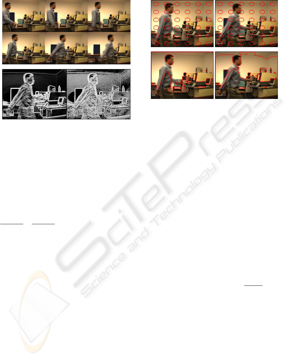
(a) Six image sequences
(b) Gradient map (c) Weight map
Figure 3: A walking man is blurred during the video record-
ing period. Background objects is unblurred with stronger
gradients edge map than the foreground people, produced
by the proposed method.
The two partition criteria in the grouping algorithm
is to minimize the disassociation between the groups
and maximize the association within the group. The
global criterion measures both the total dissimilarity
between the different groups as well as the total simi-
larity within the groups. This disassociation measure
is called the normalized cut (Ncut): Ncut(A, B)=
cur(A,B)
asso(A,V )
+
cut(A,B)
asso(A,V )
. A and B are two disjoint sets,
A ∪ B = V , A ∩ B = φ. The Lanczos method is
used to grouping similar objects which can speed up
the running time.
We extend this idea to the Mumford-Shah func-
tional for segmenting the blurred objects in video se-
quences. The reason is that the blurred objects and
unblurred objects in a degraded image have differ-
ent strength of gradients, i.e Fig. (3). The gradi-
ent edges in Fig. (3)(b) are computed using the ex-
tended Mumford-Shah regularization. The combina-
tion of low level processing and Mid or high level
knowledge can be used to either confirm these groups
or select some for further attention in repartitioning
or grouping blurred and unblurred objects in images.
The grouping algorithm is summarized as follows:
- Given a set of features, set up a undirected weight
graph G =(V, E), where V are the vertices and E
are the edges between these vertices. V can corre-
spond to pixels in an image or set of connected pix-
els. Computing the weight on each edge Fig. (3)(c),
and summarize the information into W, and D.
- Solve (D − W)x = λDx for eigenvectors with
the smallest eigenvalues.
- Use the eignevector with second smallest eigen-
(a) (b)
(c) (d)
Figure 4: The result of segmentation for a blurred walking
man using a Chan-Vese Method in two continuous images.
value to bipartition the graph by finding the splitting
point such that Ncut is maximized.
- Decide if the current partition should be subdi-
vided by checking the stability of the cut, and make
sure Ncut is below pre-specified value.
- Recursively repartition the segmented parts if nec-
essary. The number of groups segmented by this con-
trolled by the maximum allowed Ncut.
4 NUMERICAL EXPERIMENTS
4.1 Discretisation
To solve the Γ-convergence to the MS functional, we
use a discrete scheme called a cell-centered finite dif-
ference from (Vogel and Oman, 1998), (Weiser and
Wheeler, 1988). Following the way of discretization,
Eq. (9) is written in a discrete form,
2αv
ij
[(∆
x
+
f
ij
)
2
+(∆
y
+
f
ij
)
2
]+β ·
v
ij
− 1
2ε
(11)
−2βε(∆
x
+
∆
x
−
v
ij
+∆
y
+
∆
y
−
v
ij
)=0
where the forward and backward finite difference
approximations of the derivatives ∂f(x, y)/∂x and
∂f(x, y)/∂y and denoted by ∆
x
±
f
ij
= ±(f
i±1,j
−
f
ij
) and ∆
y
±
f
ij
= ±(f
i,j±1
− f
ij
). To mini-
mize the column-stack ordering of {v
ij
}, the sys-
tem is of form Mv = q, where M is symmetric
and sparse matrix and solve the minimization us-
ing Minimal residual algorithm. Let H denote the
operator of convolution of different blur PSFs that
are pre-estimated. Using the notation of (Vogel and
Oman, 1998), let L(v) denote the differential operator
L(v)f = −Div(v
2
∇f). Eq. (10) can be expressed as
H
∗
(Hu − g)+2λL(v)f =0. Let A(v)f = H
∗
f +
JOINT PRIOR MODELS OF MUMFORD-SHAH REGULARIZATION FOR BLUR IDENTIFICATION AND
SEGMENTATION IN VIDEO SEQUENCES
61
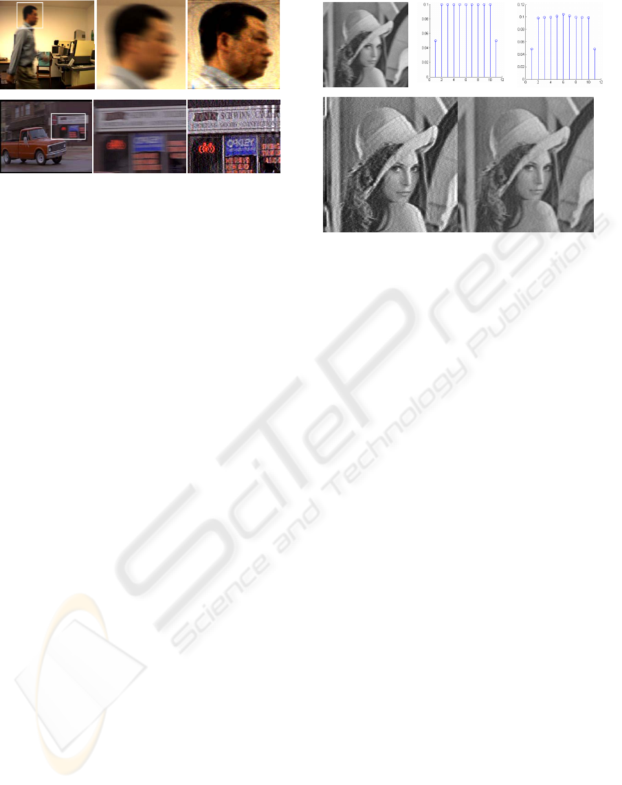
(a) (b) (c)
(d) (e) (f)
Figure 5: Blind deconvlution of degraded objects in video
sequences using estimated PSFs. (a)(d) Real video frames.
(b)(e) Blurred parts in video. (c)(f) Results of blind decon-
volution using the weighted L
2
norm regularization.
2λL(v)f, we get A(v)f = H
∗
g. f is iteratively de-
termined. To obtain f
n+1
, a correction term d
n
is
added to the current value f
n
: f
n+1
= f
n
+ d
n
× d
n
is estimated by A(v)d
n
= H
∗
g − A(v)f
n
via the
convergent descent method. Gradient edges and the
restored image are computed.
4.2 Results and Discussions
Experiments on simulated data and real data are car-
ried out to demonstrate the effectiveness of our al-
gorithm. The advantage of our method is that the
discontinuity set is not isolated closed contours. For
such cluttered images in Fig. (4), some of closed con-
tour curves using curve evolution technique (Chan
and Vese, 2001), are removed due to some boundary
leaks, stronger gradient differences, etc.
In this experiment shown in Fig. (5), we illustrate
the capability of the proposed algorithm to handle
real-life video data degraded by non-standard blur.
The video frames are captured from films or video
data with unknown shapes and sizes of the actual blur.
The degraded images are separated into RGB colour
channels and each channel is processed accordingly.
Based on the estimated PSFs and parameters in the
L
2
norm regularization approach, the accurate PSF
model helps to get the results. We also compare
the blind deconvolution results generated from the
weighted L
2
norm regularization and the Mumford-
Shah restoration. The parameters in the Mumford-
Shah functional are tuned for the best performance
α =10
−4
, β =10
−8
, ε =10
−3
with an previ-
ously estimated PSF from regularized Bayesian es-
timaion. The value of ε and β can be increased in
the presence of noise. From the results, we can found
that the Mumford-Shah functional is sharper than the
L
2
norm regularization approach using the same es-
timated PSF shown in Fig. (6). It highlights the ad-
(a) (b) (c)
(d) (e)
Figure 6: Blind restored Images from L
2
norm and MS fuc-
ntional. (a) Motion blur with 20 dB Gaussian noisy image.
(b) The original PSF. (c) The estimated PSF in 2D. (d) The
L
2
norm restored image using the estimated PSF. (e) The
Mumford-Shah restored image using the estimated PSF.
vantage of the MS functional than the weighted L
2
regularization.
The third experiment is performed using the sug-
gested method. Segmentation of a video sequences
has good performance shown in Fig. (7). Cluttered
background objects with stronger gradients do not
influence the segmentation of blurred objects with
lower gradients. The PSF is firstly blur identified. The
estimated PSF directly supports the Mumford-Shah
based segmentation to improve the accuracy of edge
detection. For the given video sequences, the PSF is
identified as a stronger motion blur. v is firstly initial-
ized as 1, the edges with some gradients are computed
after a few iterations in the extended Mumford-Shah
regularization. These detected edges are grouped via
the Ncuts method into numerical groups. The result
is labeled following the grouped regions. From the
Fig. (7), we can observe that the blurred walking man
is accurately segmented.
5 CONCLUSIONS
The paper presents a Mumford-Shah based regular-
ization using estimated PSFs prior. Blind image de-
convolution is one kind of ill-posed inverse prob-
lem. Searching for the solution in the largest space
is not a good strategy. A prior knowledge should be
used from different viewpoints to improve the solu-
tion. Support of accurate prior information directly to
the computation is an excellent strategy since the ap-
proach improves the accuracy of initial value. Using
the PSF prior, the Mumford-Shah functional is then
VISAPP 2006 - IMAGE FORMATION AND PROCESSING
62
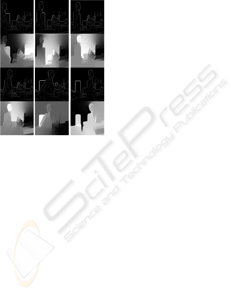
Figure 7: The results of segmentation for a blurred walk-
ing man using the MS functional and the graph-grouping
method in six continuous images.
simplified into two partial differential equations for
the image and edges and becomes more robust for
different types of blur. During the image segmenta-
tion, graph theory is integrated to partition and group
the edges driven from the Mumford-Shah functional.
These lower gradient blurred objects can then be seg-
mented accurately without any prior knowledge. It
is clear that the proposed method is instrumental in
blind image deconvolution and segmentation and can
be easily extended in practical environments.
REFERENCES
Ambrosio, L. and Tortorelli, V. M. (1990). Approximation
of functionals depending on jumps by elliptic func-
tionals via γ-convergence. Communications on Pure
and Appled Mathematics, 43:999–1036.
Aubert, l. and Kornprobst, P. (2002). Mathematical prob-
lems in image processing: partical differential equa-
tions and the Calculus of Variations. Springer.
Bertero, M., Poggio, T. A., and Torre, V. (1988). Ill-posed
problems in early vision. Proceedings of the IEEE,
76(8):869–889.
Blake, A. and Zisserman, A. (1987). Visual Reconstruction.
MIT Press, Cambridge.
Bouman, C. and Sauer, K. (1993). A generalized gaussian
image model for edge-preserving map estimation.
IEEE Transactions of Image Processing, 2:296– 310.
Chan, T. F. and Vese, L. A. (2001). Active contours without
edges. IEEE Trans. on Image Processing,, 10(2):266–
277.
Chan, T. F. and Wong, C. K. (2000). Convergence of the
alternating minimization algorithm for blind deconvo-
lution. Linear Algebra Appl., 316:259–285.
Green, P. (1990). Bayesian reconstruction from emission to-
mography data using a modified em algorithm. IEEE
Tr. Med. Imaging, 9:84–92.
Katsaggelos, A., Biemond, J., Schafer, R., and Mersereau,
R. (1991). A regularized iterative image restoration
algorithm. IEEE Tr. on Signal Processing, 39:914–
929.
Kundur, D. and Hatzinakos, D. (1996). Blind image decon-
volution. IEEE Signal Process. Mag., May(5):43–64.
Lagendijk, R., Biemond, J., and Boekee, D. (1988). Reg-
ularized iterative image restoration with ringing re-
duction. IEEE Tr. on Ac., Sp., and Sig. Proc.,
36(12):1874–1888.
Molina, R., Katsaggelos, A., and Mateos, J. (1999).
Bayesian and regularization methods for hyperpara-
meters estimate in image restoration. IEEE Tr. on S.P.,
8.
Molina, R. and Ripley, B. (1989). Using spatial models as
priors in astronomical image analysis. J. App. Stat.,
16:193–206.
Mumford, D. and Shah, J. (1989). Optimal approximations
by piecewise smooth functions and associated varia-
tional problems. Communications on Pure and Ap-
plied Mathematics, 42:577–684.
Poggio, T., Torre, V., and Koch, C. (1985). Computational
vision and regularization theory. Nature, 317:314–
319.
Rudin, L., Osher, S., and Fatemi, E. (1992). Nonlinear total
varition based noise removal algorithm. Physica D,
60:259–268.
Shi, J. and Malik, J. (2000). Normalized cuts and image
segmentation. IEEE Transactions on Pattern Analysis
and Machine Intelligence, Aug.:888–905.
Tikhonov, A. and Arsenin, V. (1977). Solution of Ill-Posed
Problems. Wiley, Winston.
Vogel, R. V. and Oman, M. E. (1998). Fast, robust total
variation-based reconstruction of noisy, blurred im-
ages. IEEE Trans. on Image Processing, 7:813–824.
Weiser, A. and Wheeler, M. F. (1988). On convergence of
block-centered finite differences for elliptic problems.
SIAM J. Numer. Anal., 25:351–275.
Zheng, H. and Hellwich, O. (2006). Double regularized
bayesian estimation for blur identification in video se-
quences. In LNCS of Asian Conference on Computer
Vision, ACCV06, pages 943–952.
JOINT PRIOR MODELS OF MUMFORD-SHAH REGULARIZATION FOR BLUR IDENTIFICATION AND
SEGMENTATION IN VIDEO SEQUENCES
63
