
ROBUST CLASSIFICATION BASED ON PRIOR OF LOCAL
DIFFERENCE PROBABILITY FOR THE UNMANNED GROUND
VEHICLES
Pangyu Jeong, Sergiu Nedevschi
Technical University of Cluj-Napoca, Computer Science Department, C-tin Daicoviciu, Cluj, Romania
Keywords: Probability features space, Bimodal Gaussian discriminator, Single class cluster center based classification,
Local Difference Probabilities (LDPs).
Abstract: The aim of this paper is to propose a new classification method based on the noise tolerant LDP (Local
Difference Probability) prior-based discriminator for the unmanned ground vehicles. This proposed
classification has three characteristics, namely, probability features space instead of Gray intensity features
space, Bimodal Gaussian discriminator (noise tolerant discriminator), and single class cluster center based
classification (only road class). Based on these components, the classification ability and classification time-
cost are better than in generic classification method; K-Mean, Fuzzy K-Mean, Contiguity K-Mean, K-Mean
applied on the texture features obtained from GMRF and from Gabor filter bank. The core of the proposed
classification is a discriminator (prior density), and it is obtained from the mean of the distances of Local
Difference Probabilities (LDPs) in the randomly selected road area. The road area is randomly selected in
front of ego vehicle, and the initial class cluster center is employed inside the sampled road area. The road
features are classified from around single cluster center to the entire image space.
1 INTRODUCTION
The technology of road detection and recognition
has dramatically developed during the last 20 years
(C. Thorpe, 1987) , (D.A. Pomerleau, 1994).
However, this research isn’t finished until now
due to the many factors impeding a good result such
as: shadow, illumination and great variations of the
road surface. These problems, however, can be
reduced, but not eliminated, when we use a road
model in order to detect the driving region (
B.
Southall, 2001)
. There are tradeoffs between using a
road model and pixel-based classification methods.
If we use a road model, we need to solve a model
selection and a model update problem. In addition it
is very sensitive in illumination. In the other aspect,
it has usage convenient and time cost advantage. If
we use a pixel-based classification, it could be
achieved in two domains like as frequency and time
domains.
In frequency domain, wavelet-based (T.R.Reed,
1990), (C. Nikias, 1991), (O. Rioul, 1991), (G.
Strang, 1989) and filter-bank-based classification (
L.
Wiskott, 1997)
, (R. O. Duda, 2001), (S.
Krishnamachari, 1997) are used in order to extract
the texture features from the image.
In time domain, the K-Mean family on the Gray
scale image is used. The K-Mean family is K-Mean,
Fuzzy-K-Mean, and Contiguity-K-Mean (J. Theiler,
1997
). These methods have considerably reduced
classification time as opposed to frequency-based
classification. However the classification time is still
not small enough for the method to be used in real-
time applications.
In another approaches, (
P. Jeong, 2003) used the
K-Mean and the local adaptive threshold method in
the combined feature vector space (
P. Jeong, 2003),
color/gray and texture, in order to classify the pixels
as road or non-road. If we use pixel classification,
we can solve the model selection problem, however,
the high time cost and road cluster merging are
required. In order to solve these problems, we
propose a new real-time pixel-based classification
method based on the Local Difference Probability
(LDP).
In Section 2, we summarize the main
characteristics of the proposed method in two
445
Jeong P. and Nedevschi S. (2006).
ROBUST CLASSIFICATION BASED ON PRIOR OF LOCAL DIFFERENCE PROBABILITY FOR THE UNMANNED GROUND VEHICLES.
In Proceedings of the First International Conference on Computer Vision Theory and Applications, pages 445-450
DOI: 10.5220/0001370604450450
Copyright
c
SciTePress

phases: learning phase, and discriminator phase. In
each phase, we explain the advantages over the
generic classification method.
In Section 3, we describe the proposed method’s
theoretical background.
In Section 4, we present the results of the
experiments.
In Section 5, the conclusion of this paper is
presented.
2 NEW FEATURE OF THE
PROPOSED METHOD
In this section, we will present the new features of
the proposed method in the learning and
discriminator points of view. These characteristics
will be explained compared to the most used
classification methods like as K-Mean, Fuzzy K-
Mean, Contiguity K-Mean, and Bayesian rule.
2.1 Learning Phase
The most important thing for the unsupervised
classification is initial cluster knowledge, and the
most important thing for the supervised
classification is prior information. The classification
ability depends on these values.
In case of K-Mean, it starts from unknown prior
information, and initial cluster center is selected
randomly or is selected in certain fixed position.
In case of the Bayesian, it starts from known
prior information. However, this information is
obtained from the previous image.
In case of the proposed method, we combined
advantages of both supervised and unsupervised
classification; we use apriori knowledge to improve
classification ability like as supervised classification,
but we obtain it from the current image like as
unsupervised classification. This helps eliminate
inaccurate prior knowledge of the Bayesian rule, and
reduces the classification time-cost by accurate
cluster knowledge in the initial stage compared to K-
Mean.
2.2 Discriminator Phase
In the case of K-Mean family and Bayesian rule, the
discriminator represents Euclidean distance for K-
Mean and Gaussian unit modal similarity for
Bayesian rule are used as a discriminator. This
makes the classification result noise sensitive.
However, in the proposed method, the discriminator
is established as a bimodal Gaussian. This makes a
classification results less noise sensitive. The
theoretical explanation of the LDP discriminator is
presented in Section 3.1.
3 THE PROPOSED METHOD
The procedure of the proposed classification method
consists of randomly selected region to obtain the
discriminator and road pixel collection based on its
value. The discriminator is described in the sub-
Section 3.1, and the classification is described in the
sub-Section 3.2.
3.1 LDP Prior Based Discriminator
The LPD prior inherits its characters from pure
Gaussian property. In order to compute class
convergence, minimum loss function based on the
“non-additive” prior is used. In case of loss function
with “non-additive” feature, the loss function can be
expressed by the quadratic loss function form.
For
m
f ℜ∈
:
)
ˆ
()
ˆ
()
ˆ
,( ffQffffL
T
−−=
where
f
is a prior function,
f
ˆ
is a expected prior
function, and
Q
is a symmetric positive-definite
)( mm
×
matrix.
The formulation of minimizing expected loss
function is rewritten according to the quadratic loss
function.
A posteriori expected loss is
)(g
PM
δ
=
)]
ˆ
()
ˆ
[(minarg ffQffE
T
f
−−
=
]}|[
ˆ
2
ˆˆ
]|[{minarg gfQEffQfgQffE
TTT
f
−+
(1)
where,
g
is an observation.
Finally, a posteriori expected loss function with
“non-additive” feature can be expressed as following
way.
)(g
PM
δ
=
PM
fgfE
ˆ
]|[ =
(2)
It still has “Posterior Mean (PM)” estimator
character, even though quadratic loss function is
used.
The LDP prior is obtained from the current
random selected region. Lets denote its components
as
VISAPP 2006 - IMAGE ANALYSIS
446

},,,{
)()2()1()( k
sss
k
s
xxxX L=
,
+
ℜ×ℜ∈
s
X
,
},{ crk ∈
(3)
where
r
is row,
c
is column in the random selected
region. And
s
indicates “sampled region”.
The LDP-based prior density at each pixel is
s
kk
k
s
k
s
x
Xp
Xp
∂
∂
=
),|(
)(
2)(
)(
σμ
}
)(
exp{)(
2
2
)(
2
)(
k
k
k
s
k
k
s
X
X
σ
μ
μ
−−
−=
(4)
where
k
μ
and
k
σ
are mean and standard
deviation obtained by 4N at each pixel position.
To achieve absolute form, power of 2 is applied
on the coefficient of exponential.
This prior density is computed only inside the
randomly selected region.
This proposed LDP-based model selection
method doesn’t need to update model in each time
stamp. It allows independent density model in each
pixel position. The model convergence is performed
in Minimum Probability Distance (MPD) like as
“Minimum loss function”. This is also proposed
method. MPD procedure is summarized as following
steps.
Step 1) Local probability distance is computed using
LDP-based prior density inside randomly selected
region. Let’s it denote as
{}
{
)()()()(
)()(
1
)(
j
s
k
s
i
s
k
s
M
k
k
d
xpxpxpxpp −+−=
=
}
M
k
m
s
k
s
l
s
k
s
xpxpxpxp
1
)()(
)()()()(
=
−+−+
(5)
where,
i
(east),
j
(west),
l
(south), and
m
(north)
are four direction neighbours (4N) of each point, i.e.,
{}
)1(,),1(),( L−kk
. And
M
is a number of used pixels
inside randomly selected region.
Step 2) Mean Distance is obtained by applying an
average on all distances obtained from current
random selected region as described below.
},,,{),|(
)()2()1(2 k
dddD
pppDp L=
σμ
,
∑
=
=
M
i
i
dD
p
M
p
1
)(
1
(6)
Step 3) New models are computed in image space.
Let’s denote image space as
},,,{
)()2()1()( k
iii
k
i
xxxX L=
,
+
ℜ×ℜ∈
i
X
,
},{ crk ∈
(7)
where
r
is row,
c
is column. And
i
indicates
“image region”.
The LDP-based density at each image pixel is
i
kk
k
i
k
i
x
Xp
Xp
∂
∂
=
),|(
)(
2)(
)(
σμ
}
)(
exp{)(
2
2
)(
2
)(
k
k
k
i
k
k
i
X
X
σ
μ
μ
−−
−≅
(8)
As we can see, a prior density and new model
density are same. Following earlier mention, this is
derived from concept of individual density model.
Step 4) Local probability distance is computed in
each image pixel using LDP-based density.
Lets it denote as
{
}
{
,)()(,)()(
)()(
1
)(
j
i
k
i
i
i
k
i
N
k
k
d
xpxpxpxpp −−=
=
}
N
k
m
i
k
i
l
i
k
i
xpxpxpxp
1
)()(
)()(,)()(
=
−−
(9)
where,
i
,
j
,
l
, and
m
are four direction
neighbourhood (4N) of each point, i.e.,
{
}
)1(,),1(),( L
−
kk
. And N is a number of used pixels in
the image space.
Step 5) MPD-based minimum loss function is
achieved by using Eq. (1).
In Eq. (1),
)(
sDs
Xpff =≡
)
: prior function obtained
from the randomly selected region.
)(
)(
i
k
di
Xpff =≡
: prior function of each pixel in the
image space. In the practical phase,
1=Q
,
0
=
ε
,
and loss function are scalar like as
0)(
2
<−
si
ff
.
Therefore the computation complexity is simple, and
the classification condition is
si
ff <
. If the pixel
satisfies this condition, it belongs to the road class.
Otherwise, it is certain that it doesn’t belong to the
road class because the proposed method only uses
one class.
3.2 Implementation of the LDP
Prior Based Discriminator
The proposed LDP-based classification is a sort of
supervised classification. The differences between
the LDP-based classification and the most used
supervised classification, namely Bayesian
classification, are that the LDP-based classification
uses current state visual information for the prior
knowledge, and that the pixels aren’t classified by
the Gaussian similarity of the pixel values, but by
the distance between the Gaussian similarities
among the pixels converted to LDP. To achieve this,
we have to solve two problems.
ROBUST CLASSIFICATION BASED ON PRIOR OF LOCAL DIFFERENCE PROBABILITY FOR THE UNMANNED
GROUND VEHICLES
447
We have to select a well-established road sample
region in order to extract prior information in current
image frame. We assume that this area is placed in
front of the ego vehicle.
We have to determine the size of road sample area.
We adopt 25% of height and 25% of width of the
image roughly because its size does not influence
much classification
Once the position and the size of the sampled road
area are determined, we have to compute the
discriminator inside it. The procedure of obtaining
discriminator starts from the noise filtering by
applying 9N averaging. Then the computation of
LDP is performed by applying 4N on the noise-
filtered pixel in sequence.
The 9N averaging and the LDP are computed at the
entire pixels of the sampled road area excepting
border of the area. This procedure is finished when
all pixels of the well-established road area are used
for calculation of the 9N averaging and the LDP
computation. Then, the distances among the LDPs
are computed. We discard the smallest and largest
distance values in the sets of distances
corresponding to the well-established sample road
area. Because we consider that it is affected by the
noise.
The average of distances is:
)(*4
)()(
)(
1
4
11
4
1
rM
kdkd
xP
r
jk
j
M
ik
i
d
−
−
=
∑∑∑∑
====
(10)
where
r
is the number of discarded distances.
“
)(xP
d
” will be used as the discriminator for
classification. It is equivalent to
s
f
in step 5.
3.3 Road Pixel Classification
Sometimes the pixels classified as road don’t cover
the entire road region because the discriminator is
computed by randomly sampling the road area (well-
established sample road region).
It means that the discriminator doesn’t satisfy all
variance of the distance between two local pixel
probabilities in the selected sample area. Therefore
we need randomly selected road area
acceptance/rejection procedures. It is achieved by
the following constraint condition.
The number of classified points has to be greater
than the number of pixels of the selected sample
area. The randomly selected road area that satisfies
equation (16) becomes the selected area for
computing discriminator.
Rji ∈
∀∀
,
,
∑∑
×
==
≥
ss
cr
j
M
i
ji
11
(11)
where
M
is a number of set of classified pixels,
and
s
r
is a row of the selected sample area and
s
c
is a
column of the selected sample area.
The initial road cluster center, one cluster center is
required, is chosen inside road area, randomly. The
classification procedure is performed in radial
direction from initial cluster center. In each radial
direction, if the distance is smaller than the distance
obtained from Equation (10), that pixel is belonging
to road class. The classification is terminated when
no pixel position moves.
Finally, road area is constructed by the contour
of the last extended pixel positions.
4 EXPERIMENTS
In this section, we will present the experiment
results in 3 different aspects.
In the 1
st
aspect, the feature vector space of
LDP are presented. This new feature vector space is
a core part of the proposed method, and it gives
many advantages in the classification phase. It is
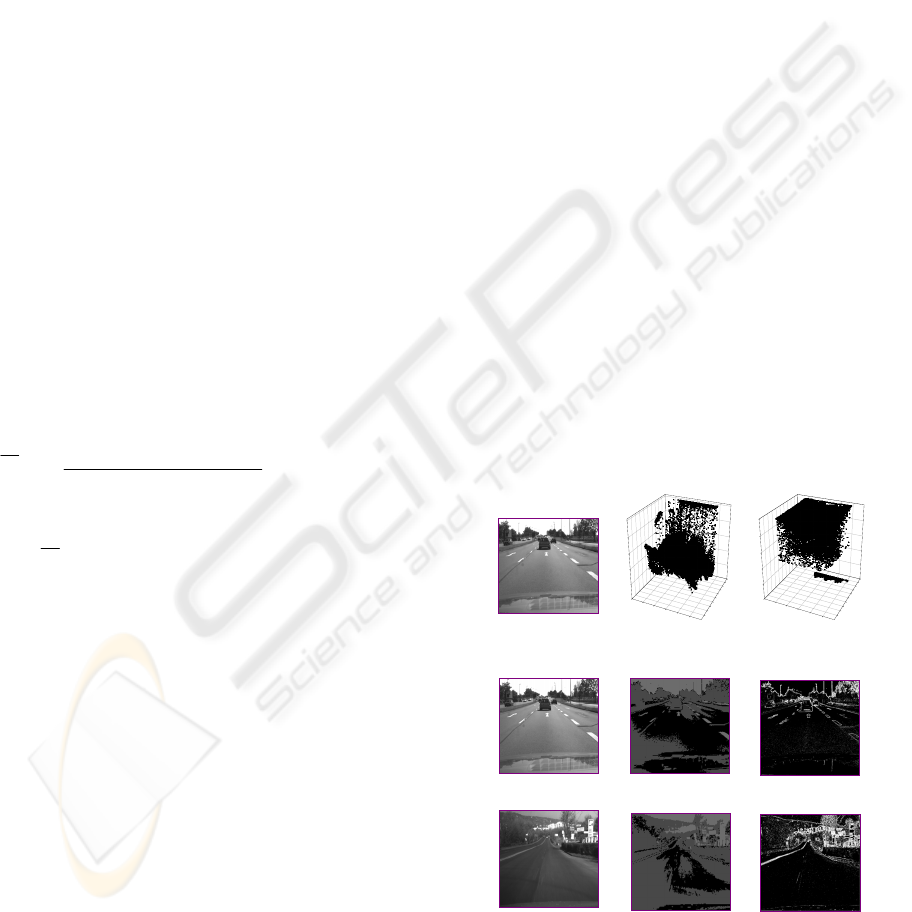
presented in Figure 1.
(b) High resolution images
[GLCM] [LDP]
[Original image]
(c) Low resolution images
[GLCM] [LDP]
[Original image]
0
50
100
150
200
250
0
20
40
60
80
100
120
140
160
180
0
50
100
150
200
G
r
a
y
i
n
t
e
n
s
i
y
f
e
a
t
u
re
v
e
c
t
o
r
s
R
o
w
C
o
l
u
m
n
0.0
0.2
0.4
0.6
0.8
1.0
0
20
40
60
80
100
120
140
160
180
0
50
100
150
200
P
r
o
b
a
b
i
l
i
t
y
f
e
a
t
u
re
v
e
c
t
o
r
s
R
o
w
C
o
l
u
m
n
(a) Feature vector space
[Original image]
[Feature vectors
generated by the LDP]
[Feature vectors in gray scale intensity]
Figure 1: The proposed new feature vector space and its
characteristic.
VISAPP 2006 - IMAGE ANALYSIS
448
In Figure 1 (a), we can notice that the LDP’s
feature vectors are concentrated from 0.8 to 1, and
the raw feature vectors of Gray image are scattered
from 0 to 200. It means that the LDP’s feature
vectors are more efficient and more robust than in
the Gray intensity feature vectors in the feature
vector grouping (road pixel classification).
Figure 1 (b) shows that how the proposed feature
vector space provides easer separation of the border
and non-border region then the generic feature
vector space. It also gives us accurate border of road
and only road class on the image.
Original image
[2 class]
[Fuzzy-Mean]
[LDP]
[K-Mean]
[4 class]
[2 class]
[4 class]
Original image
[2 class]
[Fuzzy-Mean]
[LDP]
[K-Mean]
[4 class]
[2 class]
[4 class]
(a) High resolution image
Original image
[2 class]
[Fuzzy-Mean]
[LDP]
[K-Mean]
[4 class]
[2 class]
[4 class]
Original image
[2 class]
[Fuzzy-Mean]
[LDP]
[K-Mean]
[4 class]
[2 class]
[4 class]
(b) Low resolution image
Figure 2: The comparison results of the classification
accuracy and the classification efficiency.
In the 2
nd
aspect, we present the time elapsed
during classification. This elapsed time is obtained
from relative time. It is obtained in the same testing
environment. We use a Pentium-IV 2.1Ghz CPU,
256 Mbyte memory, and 4 Mbyte graphic memory.
The results are presented in Table 1.
The proposed method doesn’t use recursive
operation; each pixel is used only one time in the
classification procedure. The algorithm iteration cost
is
)}(1|)({
crpp
nnnnO
×
≤
≤
. Where
p
n
is the
total pixel count used in the image space,
r
n
and
c
n
are row and column size of image. K-mean
family takes
)( cnnO
rc
×
×
, where c is the classifier
classes’ number. The quantity of the saved
classification time is
)()(
prc
nOcnnO −××
.
In addition we present the quantitative analysis
of the classification. The proposed method uses one
class classifier. The K-Mean family uses two classes
classifier and four classes classifier. The K-Mean
family has lots of false negative/positive error (about
43%) in two classes and (about 25%) in four classes
comparing with LDP (about 10 %). In addition the
manual road class selection is required in the K-
Mean family case. It is very difficult or it is almost
impossible to be achieved automatically. But the
proposed LDP based classification solves this
problem. The comparison results of classification
accuracy and time cost are presented in Figure 2 and
Table 1.
In the 3
rd
aspect, the segmentation ability is
presented compared to Level set (N.K. Paragios 2000)
that is the representative of region growing method
in real-time condition. It is presented in Figure 3. In
case of Level Set, the segmentation ability strongly
depends on the edge detection method. Once the
coefficient of the edge detection filter is determined
at the first image frame, it cannot be changed until
the image-processing task is finished in the image
sequence. It is shown in Level Set module in Figure
3. The segmentation ability is changed according to
different coefficient values even if the same image is
used. The used coefficient values are 0.1 (1), 0.2
Table 1: The quantitative analysis of the classification ability and the relative time cost of the classification. (3,000
images are used, and its size is 256x256).
Items
Used
classes
K-Mean
Fuzzy
K-mean
Contiguous
K-Mean
LDP
2 classes 44.82 43.51 43.3 13.6 Error (%)
(average)
4 classes 27.96 25.21 23.5
No need
2 classes 55.7 ms 500 ms 125 ms 31 ms
Time cost
(average)
4 classes 125 ms 2104 ms 250 ms
No need
ROBUST CLASSIFICATION BASED ON PRIOR OF LOCAL DIFFERENCE PROBABILITY FOR THE UNMANNED
GROUND VEHICLES
449
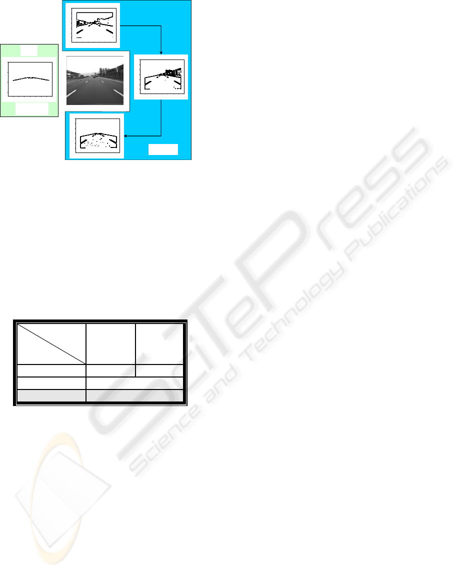
Image Width
0 100 200 300 400 500 600 700
Image Height
0
100
200
300
400
500
600
Image Width
0 100 200 300 400 500 600 700
Image Height
0
100
200
300
400
500
600
Image Width
0 100 200 300 400 500 600 700
Image Height
0
100
200
300
400
500
600
Image Width
0 100 200 300 400 500 600 700
Image Height
0
200
400
600
Auto Adapted to
Environment
Level Set
LDP
①
②
③
Image Width
0 100 200 300 400 500 600 700
Image Height
0
100
200
300
400
500
600
Image Width
0 100 200 300 400 500 600 700
Image Height
0
100
200
300
400
500
600
Image Width
0 100 200 300 400 500 600 700
Image Height
0
100
200
300
400
500
600
Image Width
0 100 200 300 400 500 600 700
Image Height
0
200
400
600
Auto Adapted to
Environment
Level Set
LDP
①
②
③
Figure 3: Comparison results of the segmentation between
Level Set and LDP.
(2), and 0.3 (3). However, the proposed LDP-
based segmentation automatically determines
classification classifier according to the feature
vector of the images at each image frame, and it
gives a key rules to keep same segmentation result in
the variant environment. In order to achieve
quantitative results, 1000 sequence images are
tested. The extension error rates are presented in
Table 2.
Table 2: The comparison of the over/under extension
ratios.
Coef. Of
Kernel
Method
0.7 0.1
Level Set ≅ 69.4 % ≅ 70.6 %
Automatic selection
LDP
≅
8.6 %
In summary of Experiments, the proposed LDP-
based classification is a more powerful method for
the road following application in the classification
cost, the classification ability, and the feature vector
space points of view.
5 CONCLUSION
We proposed the real-time classification method
based on the robust LDP-density discriminator, i.e.,
LDP prior, for the road following application of the
Unmanned Ground Vehicle (UGV). We solved the
pixel classes merging and only road class selection
problem that appeared on the road region when the
number of classes increased, and reduced the
classification cost. In addition we improved the
classification ability by using the probability feature
vector space, i.e., LDP’s feature vector space, from
Gray intensity feature vector space.
REFERENCES
C. Thorpe, T. Kanade, and S.A. Shafer, 1987. Vision and
Navigation for the Carnegie-Mellon Navlab.
Proc.
Image Understand Workshop.
D.A. Pomerleau, 1994. Reliability Estimation for Neural
Network Based Autonomous Driving. Robotics and
Autonomous Systems
.
B. Southall, C. J. Taylor, 2001. Stochastic road shape
estimation. Proceedings of the Eighth International
Conference On Computer Vision (ICCV-01)
.
T.R. Reed, H. Wechsler, 1990. Segmentation of textured
images and Gestalt organization using spatial/spatial-
frequency representations.
IEEE Trans. Pattern
analysis and Machine Intelligent
.
C. Nikias, 1991. High Order Spectral Analysis. Advances
in Spectrum Analysis and Array Processing.
S.Haykin, Ed., Prentice Hall, Englewood Cliffs, NJ
O. Rioul and M. Vetterli, 1991. Wavelet and signal
processing.
IEEE SP mag.
G. Strang, 1989. Wavelet and dilation equation: a brief
introduction. SIAMRev.
L. Wiskott, J.-M. Fellous, N. Kruger, and C. von der
Malsburg, 1997. Face recognition by elastic graph
matching.
IEEE Trans. Pattern Analysis and Machine
Intelligence
.
R.O. Duda, P.E. Hart, D.G. Stork, 2001. : Pattern
classification.
S. Krishnamachari, and R. Chellappa, 1997.
Multiresolution Gauss-Markov Random Field Models
for Texture Segmentation.
IEEE Trans. Image
Processing
.
J. Theiler and G. Gisler, 1997. A contiguity-enhanced K-
Means clustering algorithm for unsupervised
multispectral image segmentation.
Processing SPIE.
P. Jeong, S. Nedevschi, 2003. Intelligent Road Detection
Based on Local Averaging Classifier in Real-Time
Environments.
12
th
IEEE International Conference
on Image Analysis and Processing
.
P. Jeong, S. Nedevschi, 2003. Unsupervised Muliti-
classification for Lane detection using the
combination of Color-Texture and Gray-Texture.
CCCT 2003.
N.K. Paragios, 2000. Geodesic Active Contours and Level
Set methods: Contribution and Applications in
Artificial Vision.
dissertation of doctoral.
VISAPP 2006 - IMAGE ANALYSIS
450
