
REALTIME LOCALIZATION OF A CENTRAL CATADIOPTRIC
CAMERA USING VERTICAL LINES
Bertrand Vandeportaele, Michel Cattoen, Philippe Marthon
IRIT & LEN7
Enseeiht, 2 rue Camichel, 31071 Toulouse, France
Keywords:
Omnidirectional vision, localization, orientation, lines.
Abstract:
Catadioptric sensors are used in mobile robot localization because of their panoramic field of view. However
most of the existing systems require a constant orientation of the camera and a planar motion, and thus the
localization cannot be achieved in general for persons handling a camera. In this paper, we use the images of
the vertical lines of indoor environment to localize in realtime the central catadioptric camera orientation and
the 2D position. The pose detection is done in two steps. First, a two axes absolute rotation is computed to
bring the vertical line images in vertical position on the viewing sphere. Then the 2D pose is estimated using
a 2D map of the site.
1 INTRODUCTION
Our goal is to localize in realtime a central catadiop-
tric camera held by a person inside a known building.
Benosman and Kang gave in (Benosman 2001) a de-
tailed description of these cameras. They are able to
acquire instantaneously some panoramic images and
have a single viewpoint. They are frequently used in
robotic applications where the provided 360 ˚ field of
view is useful for image based localization and 3D re-
construction. Image based localization methods can
be divided in two categories:
A: methods requiring a priori knowledge about the
place where to localize the robot (for example a data-
base of appearance images corresponding to different
locations) (Padjla 2001). These methods require the
acquisition of many images and constrain the orien-
tation of the sensor. Moreover, the robust realtime
matching of occluded images is a relatively complex
problem, even if the panoramic field of view make it
easier than in the perspective case.
B: methods using Simultaneous Localization And
Mapping (Shakernia 2003). They do not require an
acquisition of the database before the localization.
Invariant points from the scene are often detected
in many images acquired at different locations using
Scale Invariant Feature Transform, KLT or Harris de-
tector, and then Structure From Motion is performed
in order to detect the position of the camera in the re-
constructed scene.
We propose a new method to achieve the localiza-
tion of a central catadioptric camera using the vertical
lines images. We use this method to localize persons.
In this application, the accuracy is not very important
(0.3m is sufficient) but the sensor can be held in dif-
ferent orientations and many occlusions can occur.
First, the vertical lines provide information about
the absolute orientation of the sensor around two axes
thanks to the common vanishing points. Second, they
can be used for localization using a simple 2D map
because they are invariant to translations about the
vertical axis. Vertical lines are numerous inside build-
ings and difficult to occlude completely. Thus, verti-
cal lines based method particulary fits our application.
Our method allows a realtime matching with vary-
ing orientation around every axes. We can use a pri-
ori knowledge consisting in a 2D map which is easy
to acquire. Thus, the camera to localize do not have
to acquire images continuously from a known starting
position. Moreover, vertical lines images are well de-
tected in varying poses and this compensates the fact
that they can be less numerous than corners in the im-
age.
In this paper, we first give a method to retrieve the
two axes orientation using the vertical lines images
acquired with a calibrated camera. Then we show
how to determine the 2D pose using a simple 2D map
of the scene and present some experimental results.
416
Vandeportaele B., Cattoen M. and Marthon P. (2006).
REALTIME LOCALIZATION OF A CENTRAL CATADIOPTRIC CAMERA USING VERTICAL LINES.
In Proceedings of the First International Conference on Computer Vision Theory and Applications, pages 416-421
DOI: 10.5220/0001370304160421
Copyright
c
SciTePress
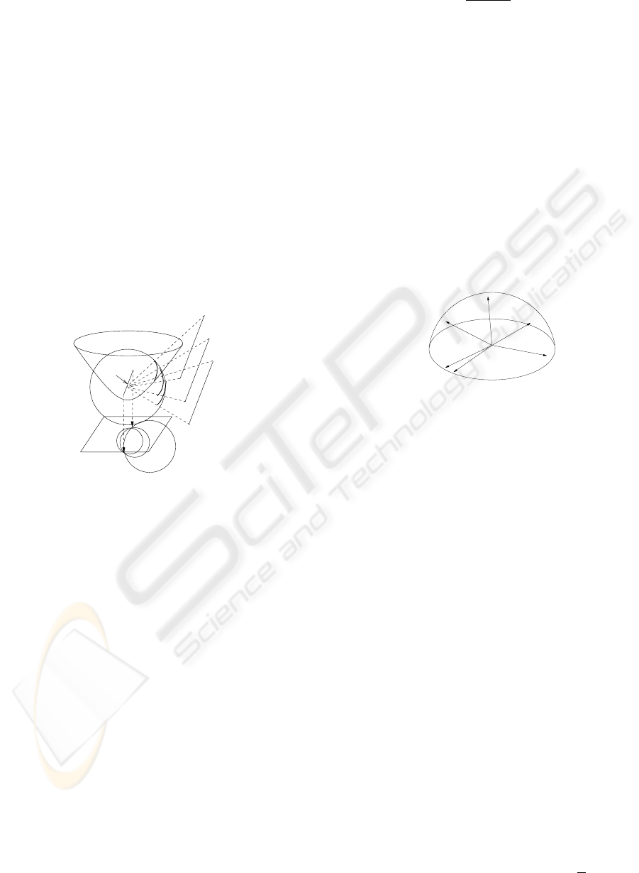
2 THE VERTICAL LINES
IMAGES DETECTION
The catadioptric camera is calibrated using the Geyer
& Daniilidis method (Geyer 1999) in order to know
the correspondence between the viewing sphere and
the image. The detection of a central catadioptric line
image di can be accomplished by finding the orien-
tation of the plane π
i
containing dli (the line image
di lifted on the viewing sphere) and the viewpoint
F as shown on fig. 1. Ying & Hu (Ying 2004) and
Vasseur & Mouaddib (Vasseur 2004) proposed robust
methods to detect the line images using a two parame-
ters Hough transform. For our experiments, we use
our own realtime line image detector which is based
on robust least squares fitting of planes on the image
points projected on the mirror surface. It provides the
same kind of results than the Hough based methods
but with increased speed.
mirror
perfect image plane
viewing
sphere
D
v
p
v1
p
v2
Q
D
1
,π
1
D
2
,π
2
D
3
,π
3
F
d
1
d
2
d
3
dl
1
dl
2
dl
3
Figure 1: Central catadioptric projection of parallel lines
to portions of great circles on the viewing sphere and the
paracatadioptric projection on the image.
The parallel lines can be detected from the image
by finding the two vanishing points located at the in-
tersection of parallel lines images which are conics
(Geyer 2001). In this case, the detection of vanishing
points is difficult because the conics parameters are
not accurately estimated from small conic sections on
noisy data and thus parallel lines images do not in-
tersect precisely in the same points (see fig 6.g for an
example).
We propose a method to gather the potentially par-
allel lines in space based on the detection of the line
D
v
which is common to a set of planes π
i
defined
by parallel lines D
i
in space. D
v
defines a bundle
of planes. In practice, the detected planes π
i
do not
intersect exactly in D
v
. Nevertheless, our method al-
lows the gathering from a criterion based on an angu-
lar measurement.
The intersection of two planes π
i
and π
j
respec-
tively with normals n
i
and n
j
is a line in the direction
h (π
i
,π
j
) passing through F . We have chosen to use
g (π
i
,π
j
), a normalized vector in the top hemisphere
defined by: g (π
i
,π
j
)=
n
i
∧n
j
||n
i
∧n
j
||
.sign
(n
i
∧ n
j
)
z
.
We give a criterion which measures how close
to a single line three planes π
i
, π
j
and π
k
inter-
sect. It uses the angular measurement ω(π
i
,π
j
,π
k
)
between g (π
i
,π
j
) and g (π
i
,π
k
): ω(π
i
,π
j
,π
k
)=
acos (g (π
i
,π
j
) .g (π
i
,π
k
)).
To deal with planes which have a normal near the
axis z, a ”close” intersection between three planes
π
i
,π
j
,π
k
is detected in the following two cases:
ω(π
i
,π
j
,π
k
) <ω
thres
or ω(π
i
,π
j
,π
k
) >π−ω
thres
.
The parameter ω
thres
is an angular threshold and has
to be set in accordance with the accuracy of the sen-
sor. On the figure 2, a small angle between g (π
1
,π
2
),
g (π
1
,π
3
) and g (π
1
,π
4
) indicates that π
1
, π
2
, π
3
and
π
4
almost define a bundle of planes so we can con-
clude that D
1
, D
2
, D
3
and D
4
are potentially parallel
in space.
F
g(π
1
,π
2
)
g(π
1
,π
3
)
g(π
1
,π
4
)
g(π
1
,π
5
)
g(π
1
,π
6
)
g(π
1
,π
7
)
Figure 2: Angles between planes intersections.
A score is given to each gathered solution by sum-
ming the scores sc
i
corresponding to planes π
i
inside
the bundle. The score sc
i
is computed for each line
image by counting the number of corresponding pix-
els. So the gathered solution having the best score
fits the greatest number of line points and thus corre-
sponds to the main orientation inside the scene.
This method is robust to erroneous detection of ver-
tical lines because the normal of such lines do not fit
inside the threshold and thus are not taken in account.
Once the planes have been gathered, a more precise
intersection is computed using iterative Levenberg
Marquardt (LM) algorithm. Let α and β be respec-
tively the azimuth and elevation of the line P
(α,β)
cor-
responding to the best intersection. Its corresponding
3D vector coordinates are P
3D(α,β)
=[P
x
,P
y
,P
z
]
and P
x
=(cos(α).cos(β)), P
y
=(sin(α).cos(β))
and P
z
= sin(β). The intersection of two random
planes from the gathered set is used as an initializa-
tion value. The different planes are weighted by their
scores sc
i
and P
3D(α,β)
is computed to be the most
possibly perpendicular line to all the weighted nor-
malized normals of planes n
i
by minimizing the fol-
lowing criteria:
C(α, β)=
sc
i
acos
P
3D(α,β)
.n
i
−
π
2
2
(1)
REALTIME LOCALIZATION OF A CENTRAL CATADIOPTRIC CAMERA USING VERTICAL LINES
417
(ˆα,
ˆ
β) = arg min
(α,β)
C(α, β) (2)
As the vertical lines are often the most numerous
inside buildings, this method is used to detect their
relative orientation and thus to detect the sensor’s ori-
entation around two axes. To increase the robustness
of the vertical line detection, we can restrict the poten-
tial orientations by asking the user to hold the camera
in an interval of angular values (±45 ˚ ). It is thus
easy to discard the candidate orientations that cannot
be vertical. The two axes orientation of the sensor is
obtained by computing the 3D rotation R(ˆα,
ˆ
β) that
brings P
3D(α,β)
to a vertical line.
3 THE 2D POSE DETECTION
Once the rotation R(ˆα,
ˆ
β) has been detected, the lo-
calization can be achieved in 2D. The altitude is not
estimated as it can vary between different users and
it is not an useful data in our application where only
an approximate localization of the camera inside the
2D map is needed. For buildings with multiple floors,
a single 2D map can be created by lifting the dif-
ferent floors maps to different locations on the same
plane. A 2D map contains the positions of vertical
lines (x
i
,y
i
) and the occlusive segments joining these
points.
In the noiseless and non degenerate cases (no more
than two map points and camera position lie on the
same line), 3 points are sufficient to localize the cam-
era. However, due to the limited accuracy of the
vertical line detector, more points should be used to
achieve an accurate localization.
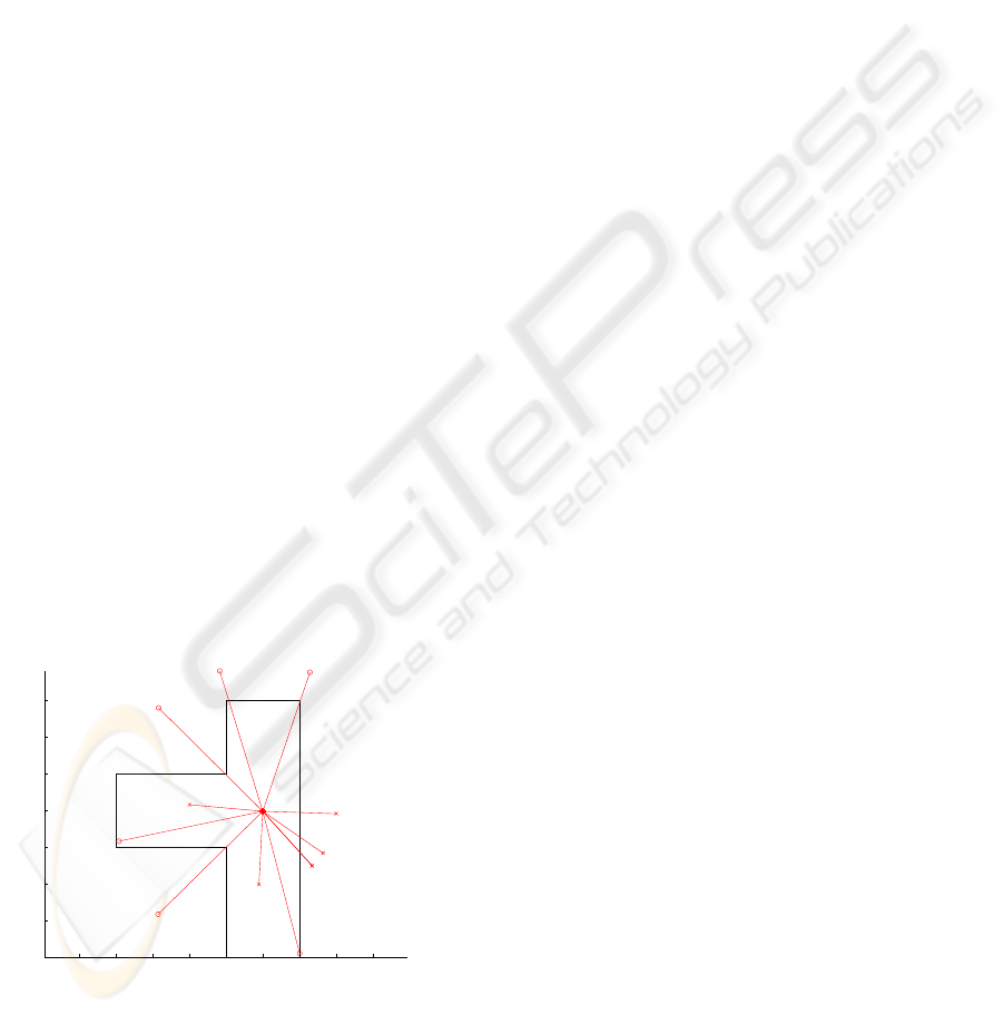
The figure 3 shows an example of a simple 2D map
made of 8 points and 8 occlusive segments.
−2 −1 0 1 2 3 4 5 6
−1
0
1
2
3
4
5
6
Figure 3: The 2D map (in black), inlier lines images (long
red lines with circles) and outliers (short red lines with
cross) after localization (the sensor is located at the inter-
section of all the red lines). The scale is in meter unit.
Each plane π
i
corresponding to a detected vertical
line is defined by an value γ
i
. γ
i
is the angle around
the vertical axis corresponding to the intersection of
the plane π
i
with the horizontal plane. The plane π
i
is not sufficient to know on which side of the view-
ing sphere lie a vertical line Di. Let p
i
be the im-
age points corresponding to the line image d
i
. These
points are lifted to the viewing sphere in P
i
and then
rotated to RP
i
= R(ˆα,
ˆ
β).P
i
in order to align the
viewing sphere with the vertical. As the p
i
correspond
to a vertical line of the scene, the RP
i
lie on the same
meridian on the viewing sphere. We use the center of
mass of RP
i
to know on which side of the sphere the
line is located and thus can compute the correspond-
ing angular value γ
i
in the range [0, 2.π]. If the RP
i
lie on the two sides of the sphere, then we detect a line
on each side of the camera. A descriptor of a location
is defined by a vector of different γ
i
.
Let us first consider that the correspondences be-
tween every γ
i
and 2D scene point i (corresponding
to a vertical line located in (x
i
,y
i
)) are known.
Let the pose be defined by three parameters. x
c
and
y
c
are the 2D position of the camera in the map and
γ
c
is the rotation.
Let γ
a
be the angular direction corresponding to the
point i in the map viewed from the pose (x
c
,y
c
,γ
c
):
γ
a
= atan2(y
i
− y
c
,x
i
− x
c
) − γ
c
(3)
The correct pose best fits the different angular val-
ues γ
a
for every γ
i
. The angular error has to be ex-
pressed in the interval [−π, π[ in order to be near
zero for small deviations in the two directions. Fi-
nally E(i, x
c
,y
c
,γ
c
) corresponds for each point i to
the squared angular difference:
E(i, x
c
,y
c
,γ
c
)=
|γ
i
− γ
a
|
[−π,π[
2
(4)
The pose is then estimated using Levenberg Mar-
quartd to minimize the following criteria:
(ˆx
c
, ˆy
c
, ˆγ
c
) = arg min
(x
c
,y
c
,γ
c
)
V
i
sc
i
E(i, x
c
,y
c
,γ
c
)
(5)
where V
i
is equal to 1 if the point i is not occluded
by segments of the map from (x
c
,y
c
) and 0 else. sc
i
is the score corresponding to the plane π
i
as described
in the previous section.
In practice, all the V
i
are equal to 1 if the correspon-
dences are all correct because only the non occluded
lines are detected on the image. If we do not deal with
the occlusions and noise and use a sufficient number
of points (> 4), the convergence is generally obtained
for any initialization value.
Let us now consider the more complex problem
of detecting inliers and outliers γ
i
and finding the
correspondences with points from the map. A sim-
ple RANSAC scheme would result in long process-
VISAPP 2006 - MOTION, TRACKING AND STEREO VISION
418
ing time even if only a few of the possible correspon-
dences have to be tested, as at least triplets (3 corre-
spondences) of couples (1 map point and one γ
i
) are
needed to compute a pose P
R
.
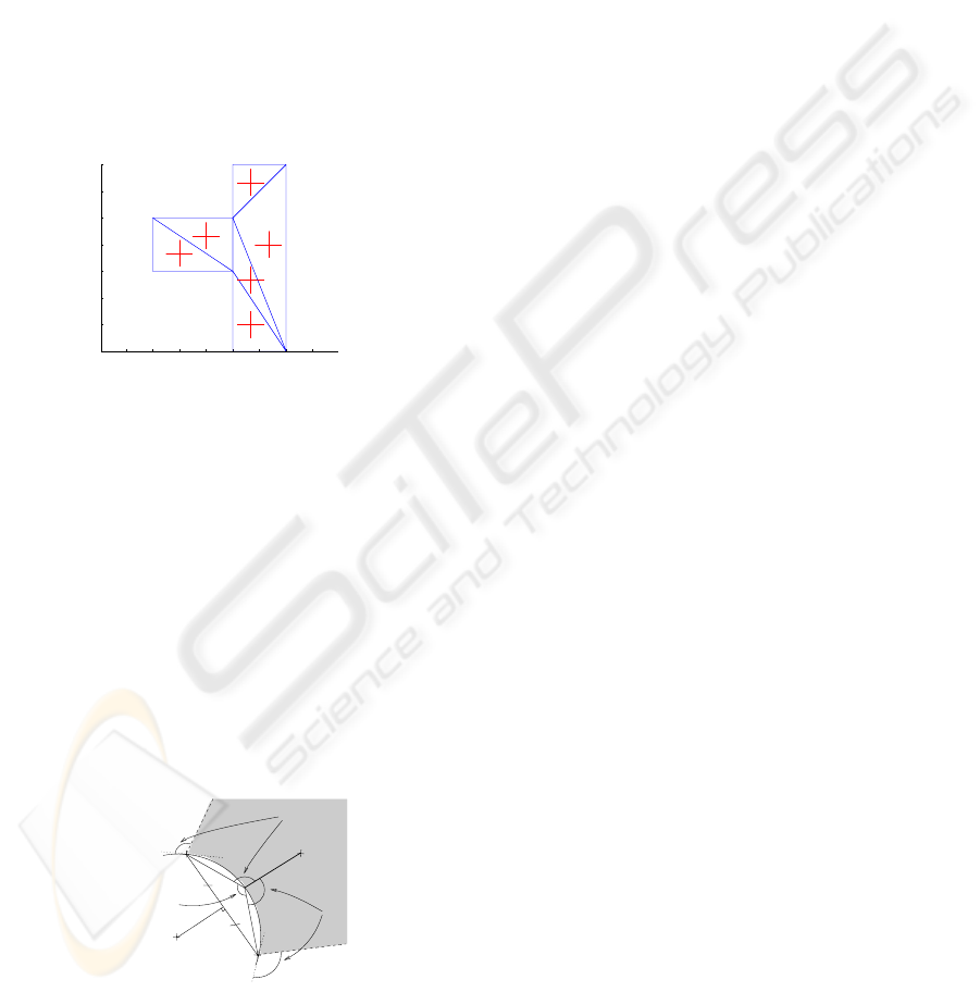
In order to reduce the computational complexity,
we propose to achieve a Delaunay triangulation of the
2D map (as shown on the fig 4). We then use the three
corners of each triangle as triplets of points to match,
as they are never occluded (by map segments) from
inside the triangle. The correspondences between the
triangle corners points i and γ
i
have to respect the or-
der constraint. If there are N map points, M values
γ
i
and P Delaunay triangles, the number of all possi-
ble solutions to test is reduced from (N.M)
3
to less
than P.M
3
as there are less than M
3
combinations of
correspondences verifying the order constraint.
−2 −1 0 1 2 3 4 5
−
1
0
1
2
3
4
5
6
Figure 4: The Delaunay triangulation of the 2D map and the
corresponding initialization value (red crosses).
We now show how to discard quickly an invalid
triplet of correspondences. Two points i and j and
a relative angle γ
i
− γ
j
define a circle of potential lo-
cations for (x
c
,y
c
) as shown on fig 5. The third point
k should lie on a line related to (x
i
,y
i
) − (x
c
,y
c
) by
γ
k
−γ
i
and to (x
j
,y
j
)−(x
c
,y
c
) by γ
j
−γ
k
. So, if the
two extremum positions are considered for the camera
position (x
c
,y
c
), (x
k
,y
k
) should lie inside the zone
between the two lines L
i
and L
j
defined by the tan-
gents of the circle at point i (resp. j) and the angles
γ
k
− γ
i
(resp. γ
j
− γ
k
). Thus, if (x
k
,y
k
) is inside the
circle or outside the zone delimited by L
i
and L
j
, the
triplet is discarded.
(x
i
; y
i
)
(x
j
; y
j
)
(x
k
; y
k
)
γ
i
− γ
j
γ
k
− γ
i
γ
j
− γ
k
center of
circle for
(x
k
; y
k
)
L
i
L
j
Figure 5: Fast detection of valid triplets (i,j,k).
The non linear optimization of the Equ. 5 is ap-
plied on the retained triplets of points in order to es-
timate the pose. The center of the Delaunay triangle
is used as initial value (fig. 4). The process is applied
to several different triplets and the pose P
R
which fits
the greatest numbers of γ
i
within an angular thresh-
old thres
γ
and without occlusion due to occluding
segments is kept.
Once the best pose P
R
has been computed from
three points, the optimization is achieved on all the
detected inliers using the pose P
R
as initialization
value.
The figure 3 shows the localization of a pose in the
2D map. The inliers are shown in red long line fin-
ishing with a circle and the outliers are shown in red
short line finishing with a cross.
Once the camera has been localized, it is easy to
track it inside the map if three lines images are visi-
ble on the two successive images. Each vertical line
projection γ
i
is tracked individually to keep the corre-
spondence information and the new pose is estimated
using the last pose as initialization value. Some corre-
spondences are removed and others are added during
the process.
4 RESULTS
In our experiments, we use 568*426 pixels images,
a paracatadioptric sensor [4] and a Pentium IV based
computer running at 1.8 Ghz. The figure 1 shows par-
allel lines imaged by this sensor. In a perfect image
plane, with zero skew and square pixels, these pro-
jections are circles having two common points (the
projections of the vanishing points p
v1
and p
v2
).
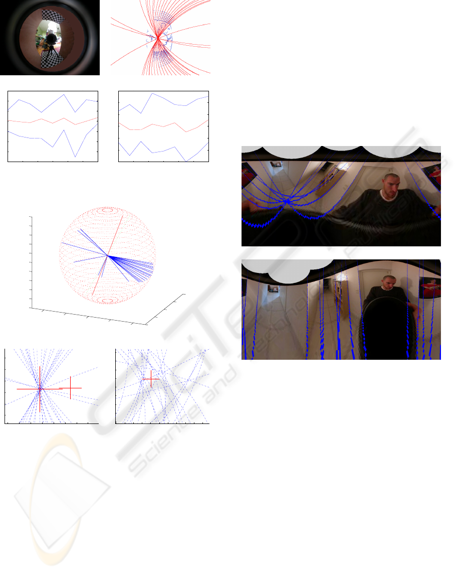
In order to validate the two axes orientation detec-
tion, the camera is mounted on a rotating table moved
by a high accuracy step motor (0.03 ˚ /step). We apply
the method to images of a scene containing two main
sets of parallel lines disposed on the 3D pattern shown
on the figure 6.a, parameter ω
thres
being set to 4 ˚.
In this example, 45 lines images have been detected.
The best set of potentially parallel lines contains 23
lines and is shown on the figure 6.b. The figure 6.e
shows the normals of planes π
i
and the correspond-
ing computed orientation (α, β) in 3D. The figures
6.f and 6.g show the two estimated vanishing points
on the paracatadioptric image plane. The orientation
of the sensor is closely related to the relative position
of the vanishing points around the projection of the
viewpoint.
We apply the method for different rotations and
plot the orientation error as a function of the real ori-
entation on the figure 6.c. 10 tests are done on dif-
ferent images for 9 different values of rotation from -
60 ˚ to 60 ˚ using a 15 ˚ step. The plot shows the maxi-
mum, minimum and mean error. The figure 6.d shows
the result for the other axis obtained by rotating the
REALTIME LOCALIZATION OF A CENTRAL CATADIOPTRIC CAMERA USING VERTICAL LINES
419
(a) (b)
−60 −40 −20 0 20 40 60
−2
−1.5
−1
−0.5
0
0.5
1
1.5
orientation in degree
angular error ( ˚ )
(c)
−60 −40 −20 0 20 40 6
0
−1.5
−1
−0.5
0
0.5
1
1.5
orientation in degree
angular error ( ˚ )
(d)
−1
−0.5
0
0.5
1
−1
−0.5
0
0.5
1
−1
−
0.8
−
0.6
−
0.4
−
0.2
0
0.2
0.4
0.6
0.8
1
(e)
240 250 260 270 280 290 300 310
1
90
2
00
2
10
2
20
2
30
2
40
(f)
1020 1040 1060 1080 1100 1120 1140 1160 1180 1200 1220
1
20
1
40
1
60
1
80
2
00
2
20
2
40
2
60
2
80
(g)
Figure 6: (a) An image of the 3D pattern. (b) Detected lines
images. (c) Maximum, mean and minimum error in degree
versus ground trust orientation. (d) Same plotting than (c)
around the other axis of rotation. (e) The normalized nor-
mals to the different planes of the bundle and the retrieved
orientation (orthogonal line ). (f) One computed vanishing
point (Big cross) and projection of the sphere center on the
image plane (Small cross). (g) The second vanishing point
(Big cross.)
3D pattern by π/2. These curves show that the esti-
mation is not biased and that the absolute maximum
deviation is less than 2˚.
Once the orientation around the two axes has been
determined, for validation purpose, a rectification of
the image is achieved in order to obtain an image from
the same viewpoint but with a fixed sensor’s orienta-
tion. The figure 7.a shows an image acquired by our
camera projected to a cylinder whose axis of rotation
is the revolution axis of the paraboloidal mirror. The
figure 7.b shows the same image projected to a ver-
tical cylinder, whose relative orientation is estimated
using the vertical lines projections. The images of the
vertical lines of the scene are approximately vertical
in the cylindrical projection, as the orientation of the
sensor has been well estimated. A completely rota-
tion invariant image can be generated by shifting the
cylindrical image by the detected orientation ˆγ
c
.
(a)
(b)
Figure 7: The cylindrical projection of the original (a) and
rectified (b) image and some of the detected vertical lines.
We now validate the 2D pose detection using the
synthetic map of the fig 3. 100 random poses are gen-
erated inside this map and 6 random inliers are kept
while 5 random outliers are added. The two first rows
of table 1 shows the mean and max absolute deviation
for the pose parameters without noise. On the first
part of the table, the γ
i
are noised. For a random an-
gular maximum deviation of 2 ˚ (which correspond to
the accuracy of our vertical lines detector), the max
pose error is less than 10cm and 2.3 ˚ . The second
part of the table shows the influence of errors in the
2D map (positions of the vertical lines) using a 2 ˚ de-
viation for γ
i
. Errors of about 20cm do not degrade
very much the accuracy of the pose estimation. The
last column shows how many poses have been com-
pletely erroneously estimated because of a bad choice
of inliers. Theses false matches are not taken into ac-
count in the calculus of the deviations.
The method is now used to localize a real camera
VISAPP 2006 - MOTION, TRACKING AND STEREO VISION
420
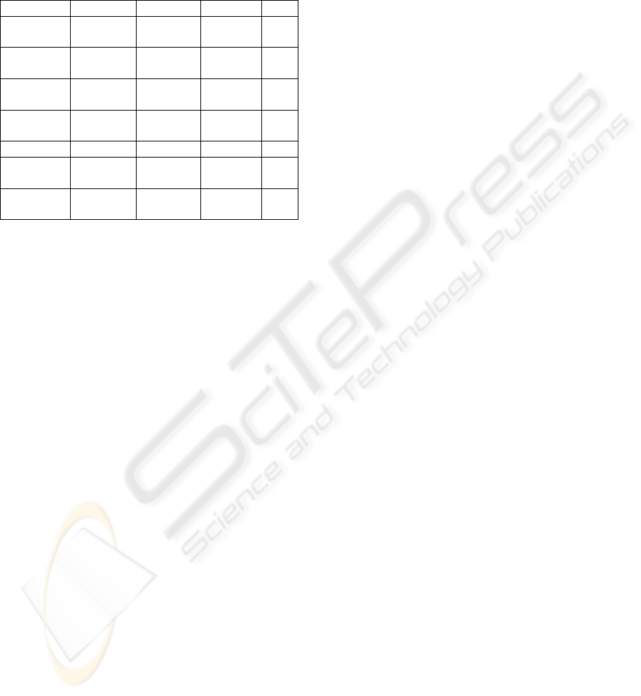
Table 1: Varying deviations of γ
i
or (x
i
,yi) over 100 tests
and their influence on the absolute deviation of pose estima-
tion parameters. (sub row 1=mean, sub row 2=max). The
right column shows the number of images that have been
erroneously localized.
∆γ
i
∆x
c
(m) ∆y
c
(m) ∆γ
c
(˚) bad
0˚ 0.0007 0.0060 0.0917 0
0.0677 0.0597 1.7762
2˚ 0.0110 0.0127 1.0485 1
0.0523 0.0998 2.3090
5˚ 0.0294 0.0305 2.4981 3
0.1743 0.1163 4.2628
10 ˚ 0.0501 0.0647 4.8415 4
0.1820 0.2830 7.3625
∆(x
i
,yi) ∆x
c
(m) ∆y
c
(m) ∆γ
c
(˚) bad
0.2m 0.0467 0.0516 1.1115 2
0.1895 0.1645 3.6326
0.5m 0.1321 0.1455 1.6100 4
0.7256 0.4124 7.7750
inside three different rooms (approx. surface: 60m2)
containing 63 main vertical lines (wall corners, win-
dows and doors borders, racks and desks) whose posi-
tions are measured by hand. The fig 7.b shows a part
of the indoor environment used in this experiment.
We processed 40 images randomly selected from a
sequence of 150 frames acquired at 15fps. 32 im-
ages were correctly localized, the position of the cam-
era being estimated inside a 20cm tolerance (We use
the tiled floor to localize approximately the camera as
ground thrust). γ
c
is compared with the angle given
by an electronic compass whose accuracy is about 2 ˚ .
The maximum detected orientation error for γ
c
in the
32 images is less than 4 ˚ . The 8 images which have
been erroneously localized can geometrically corre-
spond to different locations due to outliers. However
when we use the complete sequence to track the pose
and the correspondences between vertical lines and
γ
i
, all the 150 images are correctly localized.
The detection of the lines images takes about 40 ms
(mean time for 150 images for approx 20000 contour
points and up to 100 lines to detect). The compu-
tation of (ˆα,
ˆ
β) is generally achieved in less than 1
ms. The 2D pose estimation time greatly depends of
the complexity of the 2D map and the number of the
detected vertical lines. In our experiments, the local-
ization of the first image of the sequence has needed
1.2 sec. The tracking of the following poses, how-
ever, has been achieved in a few ms. During the first
two seconds, the computer processes the first pose and
caches the incoming images. Then it processes the
cached images more quickly than the acquisition rate
and thus can localize in realtime at 15 fps after about
three seconds of initialization.
5 CONCLUSION
In this paper, we have proposed an original method to
detect the pose of a central catadioptric camera from
an image of a indoor environment containing verti-
cal lines. The two axes orientation detection which
is first applied can be used in others applications to
detect arbitrary sets of parallel lines. The 2D pose
estimation, in spite of its apparent simplicity has ex-
hibited an high computational complexity due to the
presence of outliers and unknown matches. We have
proposed improvements allowing to achieve the pose
estimation in realtime using a smart selection of the
correspondences between the lines in the 2D map and
the detected vertical lines. Realtime is also obtained
thanks to a caching of the images and a tracking of
the correspondences inside the sequence. As future
work, we plan to integrate colorimetric information to
avoid false detections that are geometrically correct
and to accelerate the search of the correspondences
by discarding incompatible matches. Methods based
on 1D Panoramas (Briggs 2005) will also be investi-
gated. Then, experiments on entire buildings will be
achieved to validate the approach at a wide scale.
REFERENCES
X. Ying, Z. Hu (2004). Catadioptric Line Features De-
tection using Hough Transform. In Proceedings of
the 17th International Conference on Pattern Recog-
nition, volume 4, pp 839-842, 2004.
P. Vasseur and E. M. Mouaddib (2004). Central Catadiop-
tric Line Detection. In BMVC, Kingston, Sept 2004.
T.Pajdla, V.Hlavac (2001). Image-based self-localization by
means of zero phase representation in panoramic im-
ages. In Proceedings of the 2nd International Confer-
ence on Advanced Pattern Recognition, March 2001.
C. Geyer and K. Daniilidis (2001). Catadioptric Projective
Geometry. In International Journal of Computer Vi-
sion , 45(3), pp. 223-243, 2001.
C. Geyer and K. Daniilidis (1999). Catadioptric Camera
Calibration. In Proceedings of the 7th International
Conference on Computer Vision, volume 1, p. 398,
1999.
R. Benosman and S. B. Kang (2001). Panoramic Vision.
Springer, 2001.
A. Briggs, Y. Li and D. Scharstein (2005). Feature Match-
ing Across 1D Panoramas. In Proceedings of the OM-
NIVIS, 2005.
O. Shakernia, R. Vidal, S. Sastry (2003). Structure from
Small Baseline Motion with Central Panoramic Cam-
eras. In the Fourth Workshop on Omnidirectional Vi-
sion, 2003
REALTIME LOCALIZATION OF A CENTRAL CATADIOPTRIC CAMERA USING VERTICAL LINES
421
