
A NEW TECHNIQUE FOR COLOR IMAGE QUANTIZATION
Wafae Sabbar, Abdelkrim Bekkhoucha
University Hassan II Mohammedia, FST Mohammedia, Computer sciences department
BP 146 Mohammedia 20650 Morocco
Keywords: Colour image quantization; Multi-thresholding; Highpass filtering, Lowpass filtering.
Abstract: In this paper, we introduce a new technique of color image quantization. It is carried out in two processing.
In the first, we decrease the number of color using a multi-thresholding, by intervals, of the three marginal
histograms of the image. In the second processing, the colors determined in the first processing are reduced
by colors fusion based on the mean square error minimization. The algorithm is simple to implement and
produces a high quality results.
1 INTRODUCTION
Color image quantization is an important problem in
computer graphics and image processing, it is a very
useful tool for segmentation, compression,
presentation and transmission of images. It’s defined
as an irreversible image compression technique. The
main objective is to map the full color in the original
image to a much smaller palette of colors in the
quantized image by introducing a minimal distortion
between the two images (Xiang, 1994). It is very
difficult to formulate a definite solution to the image
quantization problem in terms perceived image
quality.
Mathematically, color image quantization can be
formulated as an optimization problem:
Let C={c
i
, i=1,2...N} be the set of all colors in the
image I, c
i
is a vector in one of the color spaces
(Lu*v*, HSV, RGB, ect.). A quantized image I
Q
is
represented by a set of K colors C
Q
={c
i
, i=1,2..K},
K<<N. The quantization process is therefore a
mapping:
q: C
J
C
Q
(1)
The closet neighbor principle states that each color c
of the original image I is going to be mapped into
the closet color c’ from the colour palette C
Q
:
')( ccq =
'
-min
...2,1
'-
j
cc
Kj
cc
=
= (2)
The quantization mapping defines a set of cluster
S
k/k=1,2..K
in the image color space C
{}
kk
ccqCcS =∈= )(: (3)
Color image quantization has been widely
studied for the last fifteen year, the existing
techniques of quantization can be divided into three
categories (Sangwine, 1998):
Pre-clustering algorithm: Most of the proposed
algorithms are based on statistical analysis of the
color distribution of image pixels within the color
space. The Popularity et Median Cut (Heckbert,
1982), Variance Minimization (Wan, 1990), Octree
(Gervautz, 1990) and Principal Analysis Algorithm
(Wu, 1992) are examples of this scheme.
Post-clustering algorithm: It involves an initial
selection of a palette followed by iterative
refinement of this palette using the K-Means
algorithm (Linde, 1980) to minimize the Mean
Square Error. Fuzzy C-mean (Lim, 1990) is an
extension of the K-means algorithm. The Hierarchy
Competitive Learning (HCL) (Scheunders, 1997)
and Neuuant (Dekker, 1994), exploiting the
Kohonen Self-Organizing-Maps (Kohonen, 1989]
are examples of this scheme.
Mixed algorithm: there exists a different algorithm,
which combines between the two approaches
precedent, for example the algorithm Split-Merge
described by Brun (Brun, 2000).
In this work, we propose a new method of color
image quantization witch use a multi-thresholding
followed by a merge step. The next sections are
organized as follows: In section 2 we describe the
multi-thresholding method of a marginal histogram.
In section 3 we describe our method. Experimental
results are presented in section 4. Conclusions
appear in section 5.
147
Sabbar W. and Bekkhoucha A. (2006).
A NEW TECHNIQUE FOR COLOR IMAGE QUANTIZATION.
In Proceedings of the First International Conference on Computer Vision Theory and Applications, pages 147-150
DOI: 10.5220/0001370101470150
Copyright
c
SciTePress
2 MULTI-THRESHOLDING
METHOD OF A HISTOGRAM
The objective of multi-thresholding is to devise the
histogram into a desired number of classes, every
class is represented by a peak (maximum) and
constituted by all values between two valleys
(minimum). We first evaluate the number of peaks
in the histogram, if the number of peak is more than
the desired one, we must attenuate the high-
frequency components and decrease the number of
peak by Gaussian filtering (lowpass filtering).
Otherwise, we attenuate the low-frequency
components and increase the number of peaks by
highpass filtering when the number of peaks in the
histogram is less than the desired one (Chang, 1997).
2.1 Lowpass filtering
Given a marginal histogram h(x) of an image, the
lowpass filtered L(x,
σ
) of h(x) can be obtained using
the convolution of h(x) with a Gaussian function
g(x,
σ
):
∫
−
⎥
⎦
⎤
⎢
⎣
⎡
=
x
x
d
x
hxL
μ
σ
μ
πσ
μσ
2
2
2
)-(
exp
2
1
)(),(
(4)
Where
σ
denotes de spread parameter of g and
μ
is a
dummy variable. Local maxima (peaks) and minima
(valley) of h(x) can be found from the first partial
derivate L
x
(x,
σ
) of L(x,
σ
). The peaks of L(x,
σ
) are
zero crossings in L
x
(x,
σ
) whose signs change from
plus to minus. However, valleys of L(x,
σ
) are zero
crossing in L
x
(x,
σ
) whose signs change from minus
to plus.
Let P(
σ
) denote the number of peaks in the
filtered histogram, P(
σ
) is function of the spread
parameter
σ
and decrease monotonically while
σ
increase, we must find a good
σ
to obtain the desired
number N
class
of class (peak). In order to resolving
the problem, we apply a Dichotomy method, when
the search stops, we obtained an interval of
approached value. Let
σ∗
be the upper bound of the
interval, we have two case: If P(
σ∗
)=N
class
we stop
research. If P(
σ∗
)>N
class
, we must merge P(x,
σ∗
)-
N
class
peak that gives a weak variance
2.2 Highpass filtering
When the histogram has a smaller number of peaks
than the desired number of classes, we apply a
highpass filtering. The highpass used here is
)
.2-
exp(),(
2
2
s
x
sxh =
(5)
Where the parameter s determines the bandwidth of
the stop band in the highpass filter. The highpass
filtered histogram H(x,s) of h(x) can be easily
computed in the frequency domain. We first use a
discrete Fourier Transform (DFT) to transform the
histogram h(x) to frequency domain and then apply
the highpass filter to attenuate its low frequency
components. Finally, the inverse Discrete Fourier
Transform (IDFT) is used to obtain the highpass
filtered histogram
3 QUANTIZATION METHOD
WITH THE MULTI-
THRESHOLDING BY
INTERVAL
Our method first uses a multi-thresholding, by
intervals, of the three marginal histograms h
red
, h
green
and h
blue
of the image. In the second processing, the
colors determined in the first step are reduced by
colors fusion based on the mean square error
minimization.
3.1 Multi-thresholding by interval
Each marginal histogram h
red
, h
green
and h
blue
of
image can be cut out in several intervals presented
by modes. The number of thresholds to be
determined in each interval must be proportional to
the quantity of information of this one.
We evaluates the number of peaks in each interval,
if the number of peak is more than the desired one,
we decrease the number of peak by lowpass
filtering. Otherwise, we increase the number of
peaks by highpass filtering when the number of
peaks in the interval is less than the desired one
3.2 Fusion of colour
Let C={c
0
, c
1
,..c
N
} the N produced colour by the first
processing, so we have N cluster P={C
0
,....C
N
}. If K
is the required number to quantify our image, we
must merging N-K cluster in N-K iteration. The
merge of two cluster C
i
and C
j
create a new partition
P’ with a square error E(P’) (Brun,2000).:
CμCμ
CC
CC
PEPE
2
ji
ji
ji
)(-)(
+
+)(=)'(
(6)
VISAPP 2006 - IMAGE FORMATION AND PROCESSING
148
where
∑∑
=∈
=
K
i imagec
i
cccfPE
1
-)()( (7)
and
C
CM
C
)(
)(
1
=
μ
∑
∈
=
Cc
ccfCM ).()(
1
(8)
f(c) is the number of pixels with color c in the image
and
μ(
C
)
is the means color for the cluster C.
Our merger create a graph called the Cluster
Adjacency Graph “CAG” (Brun,2000). The “CAG”
is mesh-like and has few edges that cross over each
other. Furthermore, the variance in the length of the
edges between adjacent nodes is small.
The nodes of our graph are the cluster to be
merged and each edge shared by two nodes n
i
and n
j
respectively associated to the cluster C
i
and C
j
is
valuated by
Δ(
i,j
)
:
2
)(-)(),(
ji
ji
ji
CC
CC
CC
ji
μμ
+
=Δ
(9)
If we encode the “CAG” by an half-matrix G, the
two nodes n
i
and n
j
which have be merged are
defined by:
{}{ }
]][[),(
1,...,1,...,1),(21
jiGArgMinnn
iNji ×∈
= (10)
),(]][[ jijiG
Δ
= (11)
In order to improve the search of the nodes which
have to be merged, we use an array Min defined by:
{}
{}
]][[][,......,1
1,...,1
jiGArgMiniMinNi
ij −∈
=
∈∀
The two merged nodes (n
1
,n
2
) are then defined by:
{}
⎩
⎨
⎧
=
=
∈
][
]][][[
12
,....11
nMinn
iMiniGArgMinn
Ni
(13)
Using the array Min, the computation of nodes n
1
and n
2
is performed with O(N) tests.
If we invalidate nodes n
2
, the update of this half
matrix requires to invalidate line and column n
2
and
to update line and column n
1
. The invalidation of
lines and column n
2
being performed in constant
time, this last point requires O(N) operations.
Moreover, we also have to update the value Min[i] if
Min[j] is equal to n
2
or if the update of line and
column n
1
has changed the minimum value have of
one line. In the best case where no update occurs, we
have to perform O(N-n
1
-1) tests. In the worst case,
all values Min[i] for i greater than n
1
have to be
updated. In this last case, the update of the array Min
require O(
∑
+=
−
N
ni
i
1
1
1 ) operations.
The merger needs at each node the centroid and the
cardinal of the corresponding clusters. By using
equation (8), the mean can deduced from the first
cumulative moment M
1
and the cardinal. Moreover,
as all cluster are disjoints, the first moment and the
cardinal are linear operators:
⎩
⎨
⎧
+=∪
+=∪
2121
2111211
)()()(
CCCC
CMCMCCM
(14)
As the mean can be deduced from the first moment
and the cardinal, we only store these two data in
each cluster.
4 EXPERIMENTS
In order to illustrate the results of our proposed
quantization method, we choose different images
tests very widely used in the domain of the image
processing: “Lena”(Figure 1), ”Mandrill” (Figure 2)
and “Monarch” (Figure 3), its coded in 24 bit. We
compare the new method with popular quantization
algorithm found in public domain image processing
software: Median cut, Octree and SM (Split and
Merge).These implementation worked in RGB
colors space for a fair comparison, we also use the
RGB space. The table 1 shows the distortions
produced by the quantization methods with 16 and
256 output colors. We remark that our method give
the lowest distortion for different images, the
difference is great for a quantization with 16 output
colors. Small values of distortion guarantee that a
quantization process accurately represents colors of
the original image. We notice also that the image
loses its quality from a quantization in 16 colours or
inferior.
Table1:.The distortions produced by our algorithm, SM,
Median cut and Octree.
Lena Mandrill Monarch
Nb of color
16 256 16 256 16 256
S.M
27.58 8.21 31.53 9.69 25.88 9.50
Median cut
24.65 8.23 29.54 10.55 24.67 8.66
Octree
28.08 9.46 33.02 11.50 25.58 10.58
Our meth
19.06 6.99 25.10 9.06 23.02 8.16
5 CONCLUSION
In this work we have developed a new method for
color image quantization in two processing: we use a
multi-thresholding, by intervals, of the three
marginal histograms of image in the space of color
RGB to reduce and recover the interesting color. In
order to find the required number of colors to
quantize the image, we merge the colors given a
minimal means square error using a “CAG”. The
method is simple, efficient and gives good results on
various test images.
A NEW TECHNIQUE FOR COLOR IMAGE QUANTIZATION
149
REFERENCES
Heckbert, P., 1982. Color image quantization for
frame buffer displays. Computer Graphics,
Vol.16, No. 3, 297–307.
Xiang, Z., Joy G., 1994. Color image quantization
by agglomerative clustering. IEEE Computer
Graphics and Applications, 14(3): 44-48.
Xiofan, Wu., 1992. Color quantization by dynamic
programming and principal analysis. ACM
Transactions on graphics, 11(4) : 348-
372,Octobre.
Sangwine, S. and R. Horne, 1998,The Colour Image
Processing Handbook, Chapman & Hall.
Wan, S. J., Prusinkiewicz, P., and Wong, S.K.M.;
1990. Variance-based color image quantization
for frame buffer display. Color Research and
Application, Vol. 15, No. 1, 52-58.
Gervautz, M., Purgathofer, W., 1992. A simple
method for color quantization: Octree
quantization. Graphic Gems, Academic Press,
New York (1990) 287–293.
Wu, X., 1992. Color Quantization by Dynamic
Programming and Principal Analysis. ACM
Transactions on Graphics, Vol. 11, No. 4, 348-
372.
Linde, Y., Buzo, A., Gray, R., 1980. An algorithm
for vector quantizer design. IEEE Transactions
on Communications, Vol. 28, No. 1, 84–95.
Lim,Y.W., Lee, S.U., 1990. On the color image
segmentation algorithm based on the
thresholding and the fuzzy c-means techniques.
Pattern Recognition, Vol. 23, 935-952.
Scheunders, P., 1997. A comparison of clustering
algorithms applied to color image quantization.
Pattern Recognition Letters, Vol. 18, 1379-1384.
Kohonen, T., 1989. Self-Organization and
Associative Memory, Springer-Verlag, Berlin.
Dekker, A., Kohonen, 1994. neural networks for
optimal colour quantization, Network.
Computation in Neural Systems, Vol. 5,351–367.
Brun, L., Mokhtari, M., 2000. Two high color
quantization algorithm. CGIP’2000, Saint
Etienne.
Chang, C. C., Wang, L.L., 1997. A fast multi-
thresholding method based on lowpass and
highpass filtering. Pattern recognition Letters,
181469-1478.
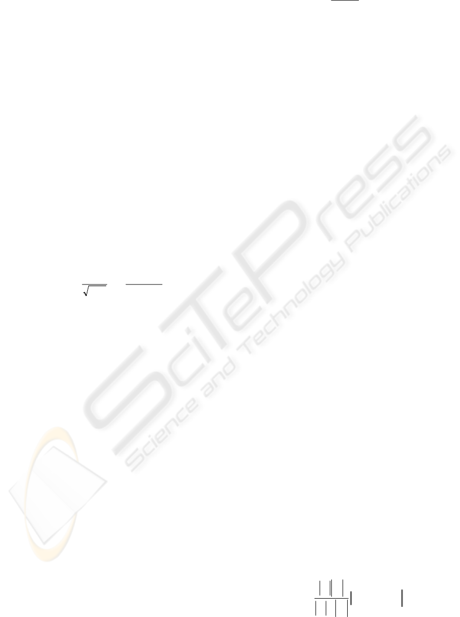
Figure 1: (the left in right) Image lenna original, image
q
uantized in 256
,
128
,
64
,
32
,
16 colours.
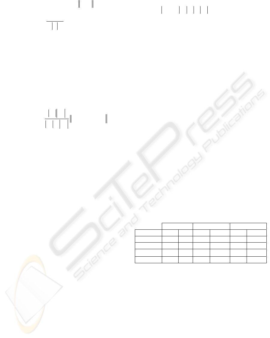
Figure 2: (the left in right) Image Mandrill original,
ima
g
e
qu
antized in 256
,
128
,
64
,
32
,
16 colours.
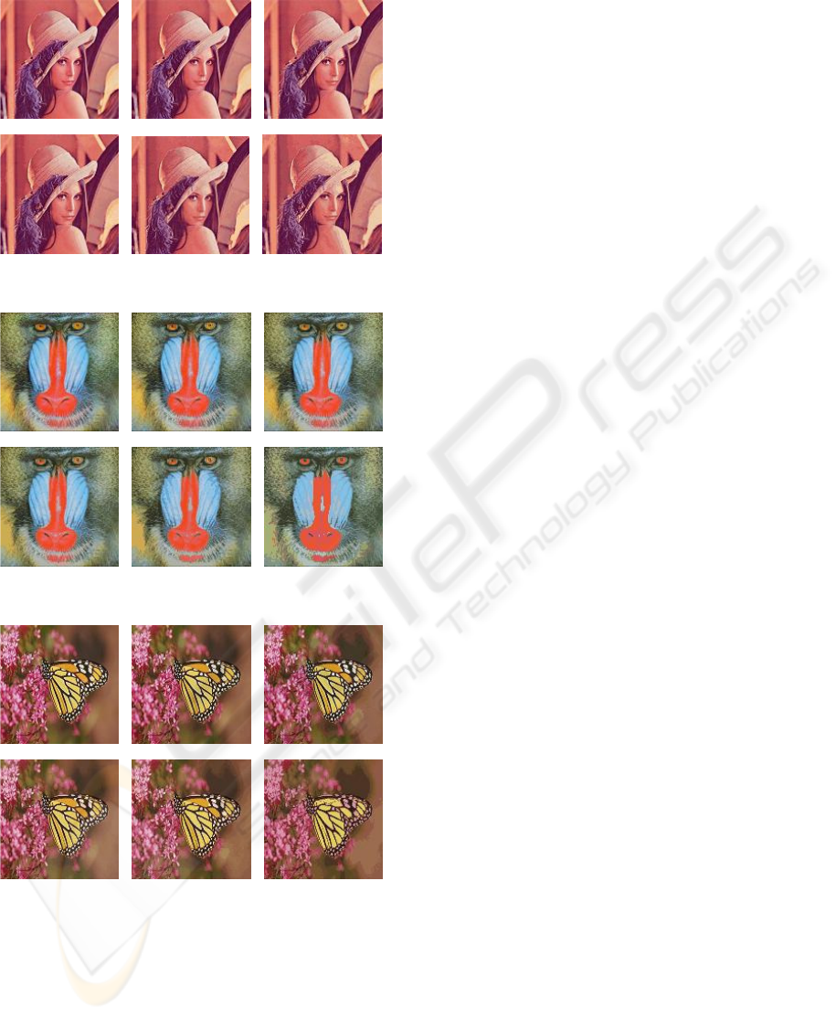
Figure 3: (the left in right) Image Monarch original,
ima
g
e
q
uantized in 256
,
128
,
64
,
32
,
16 colors.
VISAPP 2006 - IMAGE FORMATION AND PROCESSING
150
