
RENDERING (COMPLEX) ALGEBRAIC SURFACES
∗
J. F. Sanjuan-Estrada, L. G. Casado and I. Garc
´
ıa
Departament of Computer Archictecture and Electronic
University of Almeria
Ctra Sacramento s/n, 04120, Almeria (Spain)
Keywords:
Geometric computing, Roots of complex polynomials, Interval arithmetic, Rendering complex space, Ray
tracing.
Abstract:
The traditional ray-tracing technique based on a ray-surface intersection is reduced to a surface-surface in-
tersection problem. At the core of every ray-tracing program is the fundamental question of detecting the
intersecting point(s) of a ray and a surface. Usually, these applications involve computation and manipulation
of non-linear algebraic primitives, where these primitives are represented using real numbers and polynomial
equations. But the fast algorithms used for real polynomial surfaces are not useful to render complex polyno-
mials. In this paper, we propose to extend the traditional ray-tracing technique to detect the intersecting points
of a ray and complex polynomials. Each polynomial equation with some complex coefficients are called
complex polynomials. We use a root finder algorithm based on interval arithmetic which computes verified
enclosures of the roots of a complex polynomial by enclosing the zeros in narrow bounds. We also propose a
new procedure to render real o r complex polynomials in the real and the complex space. If we want to render
a surface in the complex space, the algorithm must detect all real and complex roots. The color of a pixel will
be calculated with those roots with an argument inside a selected complex space and minimum magnitude of
the complex roots.
1 INTRODUCTION
The ray tracing technique has captured its place as
an extremely valuable tool in generating photoreal-
istic synthetic imagery. Ray tracing has been inten-
sively and successfully employed to emulate specular
reflections and/or refractions, as well as to delineate
illuminated regions from those in shadow.
In ray tracing, a ray is defined as the set of points:
R =
(
x = a
x
+ t · V
x
;
y = a
y
+ t · V
y
;
z = a
z
+ t · V
z
;
)
(1)
where (a
x
, a
y
, a
z
) is the viewpoint of the scene, and
(V
x
, V
y
, V
z
) is the unit vector defining the direction
of the ray. Intersections between R and a polynomial
surface defined by f(x, y, z), is given by the set of
points in f(x, y, z) ∩ R, such that:
f(x, y, z) = f(a
x
+tV
x
, a
y
+tV
y
, a
z
+tV
z
) = 0 (2)
∗
This work has been partially supported by the Ministry
of Education and Science of Spain through grants TIC2002-
00228 and TIN2005-00447
If f(s(t)) 6= 0; ∀t ≥ 0 then f(x, y, z) ∩R = ∅ and
there is no intersection between the surface and the
ray. In the case where there exist one or more values
of t (t
0
, t
1
, . . . ; t
i
≥ 0) for which f(s(t
i
)) = 0, then
the point to visualize on the screen corresponds to the
smallest value of t
i
.
Polynomials form a fundamental class of mathe-
matical objects with diverse scientific applications.
According to the Fundamental Theorem of Algebra,
a polynomial of degree n, with real or complex coef-
ficients, has n zeros (roots) which may or may not
be distinct. The task of computing accurate zeros
of polynomials has been one of the most influential
problem in the development of several important ar-
eas in mathematics.
Computer graphics can help to visualize complex
polynomials. An good example is the visualiza-
tion software developed by Bahman Kalantari, called
polynomiography. For a given polynomial equation,
the computer applies a specific root-finding method
to a large number of zeros (z). For each initial value,
the computer determines toward which root that value
converges and assigns a colour to the point, a differ-
139
F. Sanjuan-Estrada J., G. Casado L. and Gar
´
cıa I. (2006).
RENDERING (COMPLEX) ALGEBRAIC SURFACES.
In Proceedings of the First International Conference on Computer Vision Theory and Applications, pages 139-146
DOI: 10.5220/0001369901390146
Copyright
c
SciTePress

ent colour for each root. Shades of colour indicate
how fast that point comes close to the root (Kalantari,
2004).
In this work, we propose to extend the original
ray tracing technique to complex space. Unfortu-
nately, contemporary methods for ray-tracing polyno-
mial surfaces work with real number. So it is neces-
sary to design and implement a root finder algorithm
that works with complex number.
This paper is organized as follows. Section 2
presents the algorithm to find roots of complex poly-
nomial. This algorithm uses an iterative scheme that
starts with an initial approximation of all the roots,
refines them and updates the error bound. Section 3
shows some improvements to exploit the spatial co-
herence and so to speed up the root finder algorithm.
Section 4 describes how to include these improve-
ments in ray tracing technique to render polynomial
surfaces in the complex space. Finally, several ex-
amples of real and complex polynomials rendered in
complex space are shown in Section 5.
2 ZEROS OF COMPLEX
POLYNOMIALS
In this paper, we apply the algorithm proposed in
(Hammer et al., 1995) to find a single root of the inter-
section between a complex polynomical surface and
a ray. This algorithm is based on the fact that the
roots of the complex polynomial of degree n match
the eigenvalues of the companion matrix:
A =
0 · · · 0
−p
0
p
n
1
−p
1
p
n
.
.
.
.
.
.
1
−p
n−1
p
n
(3)
Hammer showed a formulation of the Newton itera-
tion to solve the eigenvalue problem with
g
∆
q
∆
z
= −R · d + R · ∆
z
·
∆
q
0
+
(I − R · J
f
) ·
∆
q
∆
z
(4)
where matrix R is the inverse of the Jacobian matrix
(J
f
), ∆
q
is the residual value of coefficients of com-
plex polynomial, ∆
z
is the residual value of the eigen-
values, and
d = (A − ˜z · I) ·
˜q
p
n
(5)
where I is the identity matrix of dimension n, ˜q is an
approximation of the coefficients of the deflated poly-
nomial and ˜z is an approximation of the exact root of
the complex polynomial p(z).
p(z) =
n
X
i=0
p
i
· z
i
, p
i
∈ C (6)
This algorithm is structured in two parts: the Ap-
proximation and the IntervalIteration.
2.1 Approximation Algorithm
First, the Approximation algorithm improves an ini-
tial approximation ˜z of a root of a complex polyno-
mial p(z) =
P
n
i=0
p
i
· z
i
. Approximation works by
transforming the original problem to the equivalent
problem of finding an eigenvalue and its correspond-
ing eigenvector for the companion matrix A of Equa-
tion (3).
It improves the approximations of a root and the co-
efficients of the corresponding deflacted polynomial
to avoid overestimation during the floating-point in-
terval calculations. Approximation uses a residual it-
eration method to improve the initial approximation
of a root until the accuracy requirement of IntervalIt-
eration is achieved. No guarantee for the correctness
of the approximation computed by Approximation is
claimed.
In the following algorithm, the iteration
∆
(k+1)
= g(∆
(k)
) is done directly using some
loops that are equivalent to Equation (4).
Approximation(p, ˜z)
1. Termination criteria: = 10
−10
; k
max
= 50
2. Determination of an approximate eigenvector ˜q for
the initial polynomial zero ˜z
˜q
n−1
= p
n
˜q
i
= ˜q
i+1
· z + p
i+1
; for i = n − 2 to 0
3. Floating-point iteration of an eigenvalue ˜z and an
eigenvector ˜q
k = 0
(a) repeat
i. Compute the deflect d = (A − ˜z · I) · ˜q
d
0
= (−˜z · ˜q
0
− p
0
)
d
i
= (˜q
i−1
− ˜z · ˜q
i
− p
i
); for i = 1 to n − 1
ii. Compute the components of R, the inverse of
the Jacobian J
f
w
n−1
= ˜q
n−1
w
i
= (˜q
i
+ ˜z · w
i+1
); for i = n − 2 to 0
if w
0
= 0 then Err=”Inversion failed”
iii. Compute ∆
(k+1)
= g(∆
(k)
)
∆
k+1
n−1
= d
n−1
∆
(k+1)
i
= d
i
+ ˜z · ∆
(k+1)
i+1
; for i = n − 2 to 0
t = ∆
(k+1)
0
/w
0
∆
(k+1)
i
= −∆
(k+1)
i+1
+ t · w
i+1
; for i = 0 to
VISAPP 2006 - IMAGE FORMATION AND PROCESSING
140

n − 2
∆
(k+1)
n−1
= t
iv. Update ˜q and ˜z
˜q
i
= ˜q
i
+ ∆
(k+1)
i
; for i = 0 to n − 2
˜z = ˜z + ∆
(k+1)
n−1
v. k = k + 1
(b) until
||∆||
∞
max(||(
˜
(q )
n−2
i=0
||
∞
,|˜z|)
≤ or (k = k
max
)
4. Return ˜q, ˜z, Err
We use k
max
= 50 as the maximum number of
iterations, and = 10
−10
as the value for the rela-
tive error. If the condition number of the inverse R is
extremely large, then the convergence of the residual
iteration is slow. To avoid the possibility of an un-
bounded number of iterations at step 3, we halt after
k
max
iterations. It turned out that k
max
and are good
values for minimizing the effort to get sufficiently ac-
curate approximations of ˜z and ˜q.
2.2 Interval Iteration Algorithm
The algorithm IntervalIteration computes a verified
enclosure of a root of a complex polynomial using
an interval iteration. Starting with good approx-
imations ˜z for a root of the complex polynomial
p(z) and ˜q for the coefficients of the deflated
polynomial q(z) =
p(z)
z−˜z
, a verification strategy
based on Schauder’s fixed-point theorem is used to
determine (if possible) a guaranteed enclosure of a
polynomial root z
∗
(Granas and Dugundji, 2004) and
(Jimenez-Melado and Morales., 2005). In addition,
guaranteed enclosures of the coefficients of the
deflated polynomial q
∗
(z) =
p(z)
z−z
∗
are returned.
IntervalIteration(p, ˜z)
1. Computation of the interval evaluation
(a) Compute an enclosure of d (Eq. (5))
[d]
0
= (−˜z · ˜q
0
− p
0
)
[d]
i
= (˜q
i−1
− ˜z · ˜q
i
− p
i
); for i = 1 to n − 1
(b) Compute an enclosure of [R], the inverse of the
Jacobian J
f
[w]
n−1
= ˜q
n−1
[w]
i
= (˜q
i
+ ˜z · [w]
i+1
); for i = n − 2 to 0
if 0 ∈ [w]
0
then Err=”Verified enclosure failed”
(c) Compute enclosures of ∆
(0)
q
and ∆
(0)
z
[∆]
(0)
n−1
= d
n−1
[∆]
(0)
i
= [d]
i
+ ˜z · [∆]
(0)
i+1
; for i = n − 2 to 0
[t] = [∆]
(0)
0
/[w]
0
[∆]
(0)
i
= −[∆]
(0)
i+1
+ [t] · [w]
i+1
; for i = 0 to
n − 2 [∆]
(0)
n−1
= [t]
2. Interval iteration
k = 0; = 10
−1
; k
max
= 10
(a) Repeat
i. Slightly enlarge the enclosure interval
[∆]
(k)
= [∆]
(k)
ii. Determine a new enclosure interval of (4)
[v]
n−1
= 0
[v]
i
= ([∆]
(k)
n−1
·[∆]
(k)
i
+˜z·[v]
i+1
); for i = n−2
to 0
[v]
0
=
[v ]
0
[w]
0
[∆]
(k+1)
i
= ([∆]
(0)
i
+ [v]
i+1
− [v]
0
· [w]
i+1
) for
i = 0 to n − 2
[∆]
(k+1)
n−1
= [∆]
(0)
n−1
− [v]
0
iii. k = k + 1
(b) until ([∆]
(k)
⊂ [∆]
(k−1)
) or (k = k
max
)
3. Verification of the result
if ([∆]
(k)
⊂ [∆]
(k−1)
) then
[q]
i
= (˜q
i
+ [∆]
(k)
i
); for i = 0 to n − 2
[q]
n−1
= p
n
[z] = (˜z + [∆]
(k)
n−1
)
else Err=”Inclusion failed”
4. Return [q], [z], Err
We use k
max
= 10 as the maximum number of
iterations, and = 0.1 as the value for the epsilon
inflation. It turned out that these are good values for
minimizing the effort if no verification is possible.
2.3 CAllPolyZero Algorithm
Hammer et al. designed an algorithm for finding a sin-
gle complex root (CPolyZero) which uses algorithms
Approximation and IntervalIteration (Hammer et al.,
1995). Because of our interest in finding all the com-
plex and real roots of polynomial, we have designed a
new algorithm called CAllPolyZero. By repeating the
deflation of a verified zero from the reduced polyno-
mial pdef lated[q], the approximation of a new zero
in the reduced polynomial and the verification of the
new zero in the original polynomial, we get all simple
zeros of the polynomial. The new deflated polyno-
mial is computed by the algorithm IntervalIteration
based on the current value of [q]. For approximating a
new zero, the deflated polynomial pdeflated is used.
The verification of the new zero is done in the orig-
inal polynomial p because zeros of the approximate
deflated polynomial are smeared out because [q] has
interval-valued coefficients, while p has point-valued
coefficients.
AllCPolyZeros(p, ˜z)
1. pdeflated = p
2. for i = 1 to n − 1 do verification of a new zero
(a) Approximate a new zero of pdeflated:
Approximate(pdeflated, ˜z)
RENDERING (COMPLEX) ALGEBRAIC SURFACES
141
(b) Verify the new zero for p
(c) Deflate verified zero from pdeflated
This algorithm finds all roots of complex and real
polynomials. If AllCPolyZeros algorithm works with
a real polynomial (imaginary part of each coefficient
is zero) and a real initial approximation of ˜z ∈ R, it
will never get enclosures of a pair of conjugate com-
plex zeros of p(z), because all complex arithmetic op-
erations deliver a real result. However, for finding
a complex conjugate zero of a real polynomial, All-
CPolyZeros algorithm must start with a non-real ini-
tial approximation ˜z.
3 SPATIAL COHERENCE
In this section, some improvements to speed up of
CAllPolyZero algorithm are shown. This algorithm
needs an initial approximation ˜z to start the process.
If this parameter is near to the exact root then it is nec-
essary a few number of iterations. This means that is
necessary to supply a good initial approximation ˜z to
reduce the algorithm execution time.
Numerous optimization methods for ray tracing
have been suggested since it was first introduced
(Whitted, 1980). Many have suggested the exploita-
tion of spatial coherence (Glassner, 1989). Once a
single ray has been processed, a ray emitted for a
nearby pixel at a similar direction will hit, most likely,
a nearby target. We propose to exploit spatial coher-
ence, so that if a primary ray hit a surface in pixel
(j, k), it is very probable that the primary rays of
neighboring pixels hit the same object. These neigh-
boring pixels are (j−1, k−1), (j, k−1), (j+1, k−1),
(j − 1, k), (j + 1, k), (j − 1, k + 1), (j, k + 1) and
(j + 1, k + 1).
In order to find the initial approximation of the root
associated to pixel (j, k), we propose to choose the
average value of the roots in the neighboring pixels.
Following, we show how to compute this average ini-
tial approximation ˜z for pixel (j, k):
1. CAllPolyZero only can use the roots associated to
pixels: (j − 1, k − 1), (j, k − 1), (j + 1, k − 1) and
(j − 1, k). Notice that the roots associated to the
remaining neighboring pixels have not been com-
puted yet.
2. If a primary ray does not hit an object in a neighbor-
ing pixel, then this pixel is not used in this average.
3. If every primary rays of neighboring pixels does
not hit an object then the initial approximation ˜z is
0 + i.
4. If several primary rays of neighboring pixels hit
some objects:
(a) If the primary rays hit the same object, we cal-
culate only a single average value of the initial
approximation.
(b) If the primary rays hit several objects, several
average values of the initial approximations are
computed, one for each object.
4 RAY TRACING IN COMPLEX
SPACE
The previous sections describes our general algorithm
for computing all roots of a polynomial, and compu-
tations are done in the complex space. In this section,
we will briefly describe the technique used to com-
pute the colour of each pixel in an image rendered
by ray tracing techniques. The traditional ray tracing
uses the minimum positive root to assign the colour of
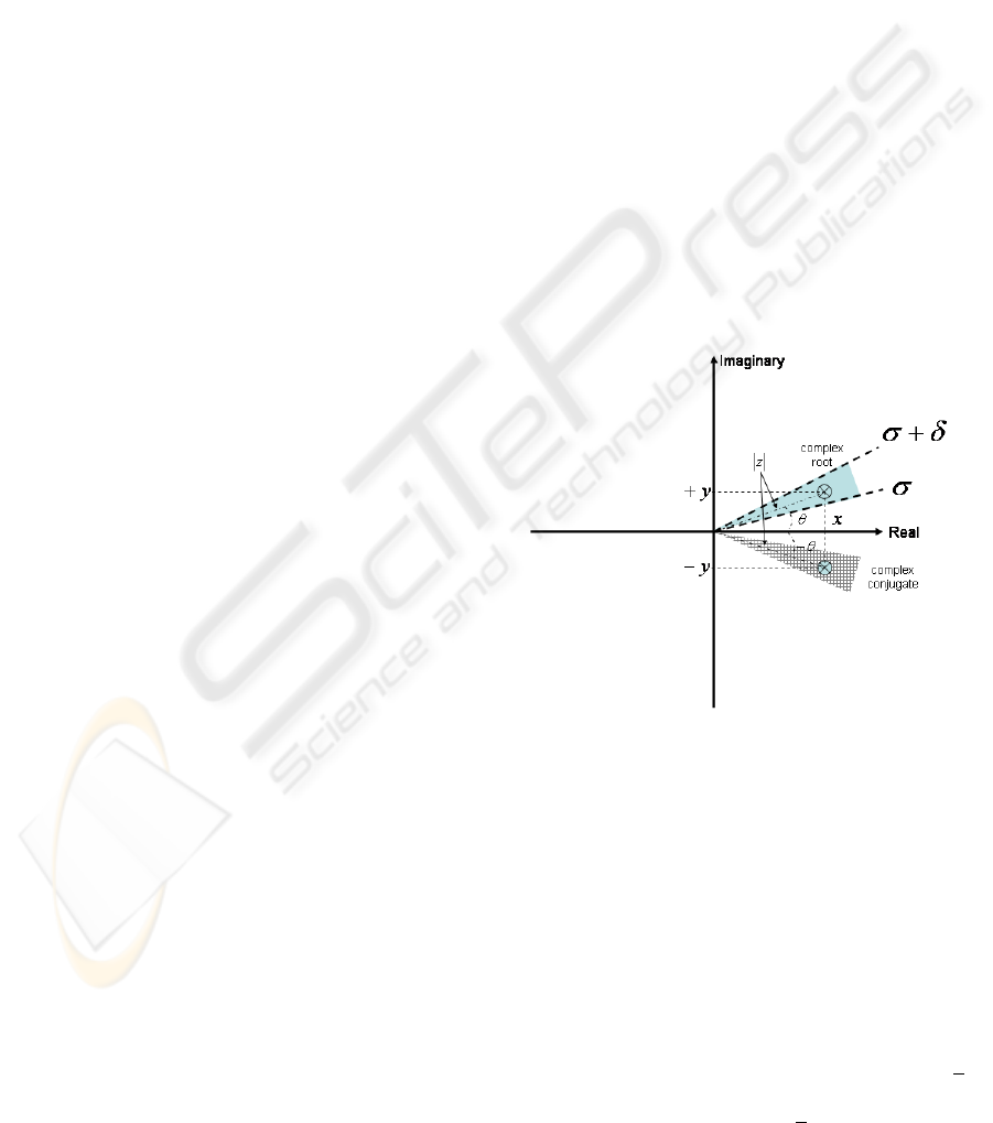
a pixel in real space. A complex number z = x + i · y
can be represented in complex space, like ρ · e
i·θ
, the
magnitude represents its modulus ρ and the angle θ its
complex argument (see Figure 1).
Figure 1: Sampling complex space.
In our algorithm the selected root is that with the
minimum magnitude and with its complex argument
θ in a selected range given by σ ≤ θ ≤ σ + δ. The
selected root will determine the final colour of a pixel.
This means that the rendering process is guided not
only by the magnitude of the roots but also it can play
with their complex arguments. This algorithm will
allow to sample the complex space, so that different
images can be obtained by choosing the interval angle
[σ, σ + δ] (see Figure 1). For example, for rendering
a scene in the real space, σ = 0 and δ = 10
−10
are
appropriate values. However, for σ = 0.1 and δ =
π
4
,
the selected roots belong to the complex space with
angles between 0.1 ≤ θ ≤ 0.1 +
π
4
and their complex
VISAPP 2006 - IMAGE FORMATION AND PROCESSING
142

conjugate −0.1 −
π
4
≤ θ ≤ −0.1. In this case, the
real roots are not included in the search space.
This procedure allows us to render three-
dimensional complex algebraic surfaces in the
complex space with an angle bounded. For rendering
all complex space using ray tracing, we can sample
all space with different values of δ and σ. Due to the
symmetry of the conjugate complex roots, it is only
necessary to sample the complex space determined
by σ ≥ 0 and σ + δ ≤ π .
When we render a scene defined by complex alge-
braic surfaces, we can use a maximum δ value equal
to π (and σ = 0). The result is that we obtain a large
amount of roots associated to the same pixel because
we are dealing with the full complex space. Our pro-
posal consists of sampling the complex space with a
narrow aperture angle; i.e. small values of δ. This
method allows us to generate an animated sequence
of images, each corresponding to a different value of
δ. The animated sequence of images gives an interest-
ing information about the distribution of roots in the
complex space.
5 EXPERIMENTATION
We use the C-XSC library, a C++ class library for eX-
tended Scientific Computing, to implement the pro-
posed algorithm. Its wide range of numerical data
types, operators and functions for scientific compu-
tation makes C-XSC especially well suited as a speci-
fication language for programming with automatic re-
sult verification.
The automatic verification of the numerical results
is based on interval arithmetic. The easiest technique
for computing verified numerical results is to replace
any real or complex operation by its interval equiva-
lent and then to perform the computations using in-
terval arithmetic. This procedure leads to reliable and
verified results. However, the diameter of the com-
puted enclosures can be as wide as to be practically
useless. We have applied the principle of iterative re-
finement (IntervalIteration) to our algorithm, which
will allow us to compute an interval error less than a
desired accuracy. The verified enclosure of the solu-
tion is given by the approximation of the root and the
enclosure of its error.
In order to observe the performance of our algo-
rithm, we have used a set of polynomials with more
than twenty different polynomials. However, in this
paper, we only show six interesting polynomials due
to space limitations (see Table 1).
The CAllPolyZero algorithm needs the coefficients
of polynomial obtained by Equation (2) to transform
f(x, y, z) in an univariate polynomial f(t). So that,
the sphere polynomial is p
2
· t
2
+ p
1
· t + p
0
, while the
Table 1: Polinomial surfaces.
Surface Polynomial equation f(x, y, z)
Sphere x
2
+ y
2
+ z
2
− 1
Whitney x
2
· z + y
2
Steiner x
2
· y
2
+ x
2
· z
2
+ x · y · z + y
2
· z
2
Chair x
4
− 1.2 · x
2
· y
2
+ 3.6 · x
2
· z
2
+
16 · x
2
· z − 7.5 · x
2
+ y
4
+
3.6 · y
2
· z
2
− 16 · y
2
· z−
7.5 · y
2
− 0.2 · z
4
− 7.5 · z
2
+ 64.0625
Tangle x
4
− 5 · x
2
+ y
4
− 5 · y
2
+ z
4
− 5 · z
2
+ 11.8
Boy −729 · x
6
+ 1374.6156 · x
5
· z−
2187 · x
4
· y
2
− 810 · x
4
· z
2
+ 324 · x
4
· z−
2749.23 · x
3
· y
2
· z − 305.47 · x
3
· z
3
−
2187 · x
2
· y
4
− 1620 · x
2
· y
2
· z
2
+
648 · x
2
· y
2
· z + 1832.82 · x
2
· y · z
3
−
1832.82 · x
2
· y · z
2
+ 324 · x
2
· z
4
−
144 · x
2
· z
2
− 4123.85 · x · y
4
· z+
916.41 · x · y
2
· z
3
− 729 · y
6
−
810 · y
4
· z
2
+ 324 · y
4
· z − 610.94 · y
3
· z
3
+
610.94 · y
3
· z
2
+ 324 · y
2
· z
4
−
144 · y
2
· z
2
− 216 · y + 432 · z
6
− 288 · z
5
+
64 · z
4
Whiney polynomial is p
3
· t
3
+ p
2
· t
2
+ p
1
· t + p
0
and
p
4
·t
4
+p
3
·t
3
+p
2
·t
2
+p
1
·t+p
0
for Bicube, Steiner,
Chair and Tangle polynomials. Finally, the degree of
Boy polynomial is six, like p
6
· t
6
+ p
5
· t
5
+ p
4
· t
4
+
p
3
· t
3
+ p
2
· t
2
+ p
1
· t + p
0
.
Figures 3 and 4 show a sphere where only p
0
is
a complex coefficient. Both images are different be-
cause the first one was rendered for σ = 0 and
δ =
π
18
, while δ =
7·π
18
in the second one. It is im-
portant to see how the complex roots transform a real
sphere (see Figure 2) in a sphere with special effects.
These effects can modify the texture, size and illumi-
nation of the surface.
The Tangle polynomial was rendered in real (see
Figure 2: Sphere polynomial where all coefficients are real
numbers. This image was rendered in real space for σ = 0
and δ = 0.
RENDERING (COMPLEX) ALGEBRAIC SURFACES
143
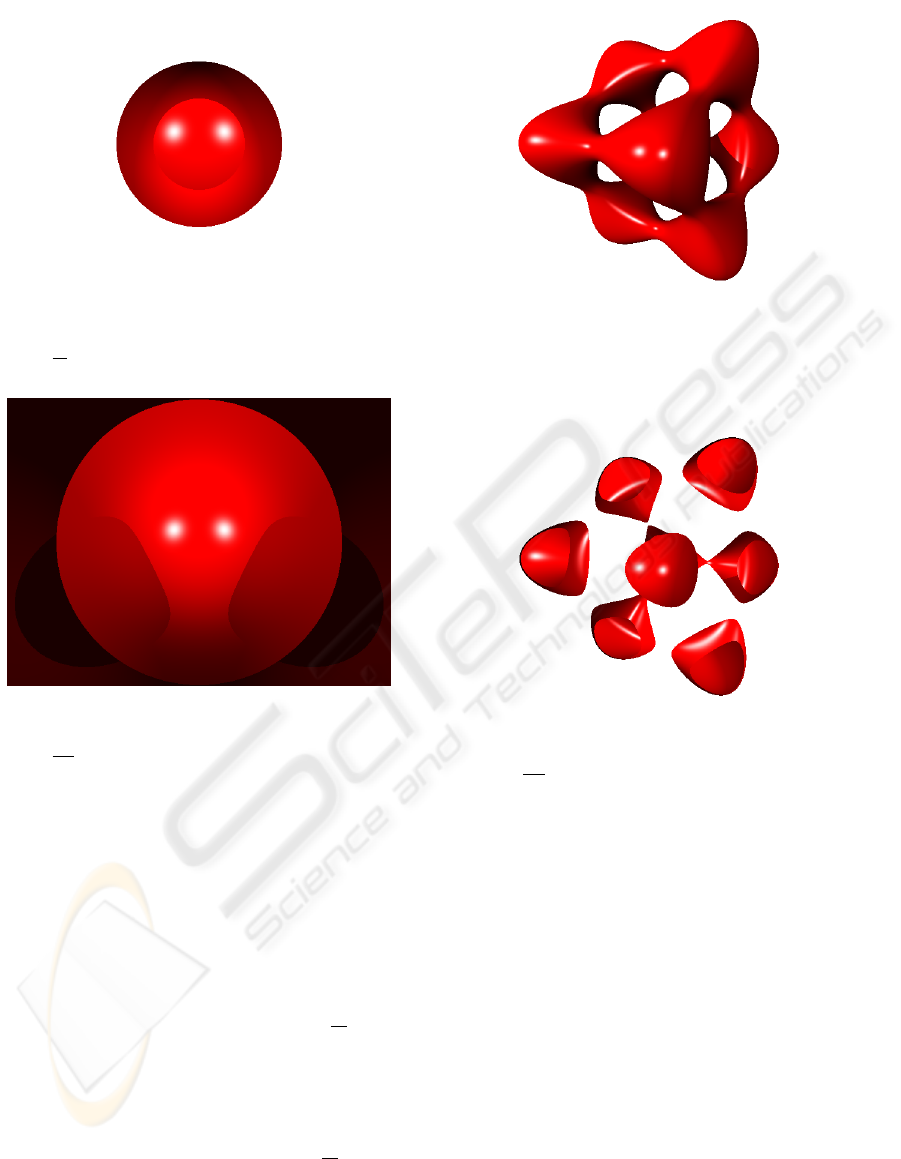
Figure 3: Sphere polynomial where p
0
is a complex coeffi-
cient. This image was rendered in complex space for σ = 0
and δ =
π
18
.
Figure 4: Sphere polynomial where p
0
is a complex coeffi-
cient. This image was rendered in complex space for σ = 0
and δ =
7·π
18
.
Figure 5) and complex space. The images rendered
in complex space were represented by p
0
(see Fig-
ure 6) and p
2
(see Figure 7) as complex coefficient.
All these images show big differences. On one hand,
same pieces of real surface disappear in the complex
space, as shown in Figure 6. On the other hand, it
is very interesting to highlight the shadows appearing
on the Tangle surface (see Figure 7).
Figure 9 shows the Whitney polynomial rendered
in the complex space for σ = 0 and δ =
π
18
. When
p
0
is a complex coefficient then some shadows ap-
pear on the image. These shadows are very different
from Whitney polynomial rendered in real space (see
Figure 8). However, a new piece of surface around
imaginary axis of Whitney surface appears when we
sample the complex space between 0 and
π
18
.
The following sequence of images for Steiner sur-
face is very interesting. The complex roots of this
surface do not cover the object, but they are located
around three ”imaginary” axes of surfaces. For exam-
Figure 5: Tangle polynomial where all coefficients are real
numbers. This image was rendered in real space for σ = 0
and δ = 0.
Figure 6: Tangle polynomial where p
0
is a complex coeffi-
cient. This image was rendered in complex space for σ = 0
and δ =
π
180
.
ple, the Steiner surface shows the three axes which ap-
pear in the complex space (see Figure 10). It is impor-
tant to show that this sequence is obtained sampling
the complex space, so that this allow us to analyse the
evolution of the complex roots for the Steiner surface.
Finally, we have rendered a sequence of images for
the Boy surface (see Figure 11). This sequence begins
with a representation of the Boy surface with all co-
efficients in real space and rendered in the real space.
Later the Boy surface with p
0
, p
1
, p
2
, p
3
and p
4
as
complex coefficients were rendered in complex space.
This example shows how the surface is disappearing
around the real axis of complex space when the co-
efficient higher is a complex number. In this case,
the Boy surface completely disappear around real axis
when p
5
or p
6
are complex coefficients. That means
that complex roots for these coefficients are far from
real axis.
VISAPP 2006 - IMAGE FORMATION AND PROCESSING
144
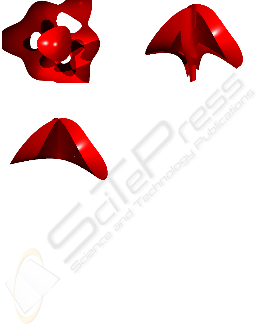
Figure 7: Tangle polynomial where p
2
is a complex coeffi-
cient. This image was rendered in complex space for σ = 0
and δ =
π
18
.
Figure 8: Whitney polynomial where all coefficients are
real numbers. This image was rendered in real space for
σ = 0 and δ = 0.
6 CONCLUSION
We have designed and implemented a complex root
finder algorithm to render complex polynomial sur-
faces in complex space. For this problem, it is not
possible to use the Sturm sequences of a complex
polynomial as a root finder algorithm. This is due to
some of the polynomial coefficients are complex and
additionally we are interested in the complex roots of
the intersection. We solve this problem as an eigen-
value problem, where we have used the polynomial
root finding algorithm proposed by Hammer with
some additional extras. On the one hand, we have
solved the problem of distinguishing zeros which are
very close one to each other with high accuracy. On
the other hand, we have extended this algorithm to
find all the complex roots associated to each pixel of
the rendered image.
Finally, we have proposed a new procedure to ren-
der images with a ray tracing technique in the com-
Figure 9: Whitney polynomial where p
0
is a complex co-
efficient. This image was rendered in complex space f or
σ = 0 and δ =
π
18
.
plex space. This technique allows us to build a se-
quences of images from which we can analyse the
evolution of the complex roots of several complex
and real polynomial surfaces in a three-dimensional
space. The typical effects of rendering real surfaces
such as reflection, refraction or translucent can also
be applied to rendering complex algebraic surfaces.
REFERENCES
Glassner, A. (1989). An Introdu ction to Ray Tracing. Aca-
demic Press, Boston.
Granas, A. and Dugundji, J. (2004). Fixed point the-
ory. Bulletin of the American Mathematical Society,
41(2):267–271.
Hammer, R., Hocks, M., Kulisch, U., and Ratz, D. (1995).
C++ Toolbox for Verified Computing I: Basic Numer-
ical Problems: Theory, Algorithms, and Programs.
Springer-Verlag, Berlin.
Jimenez-Melado, A. and Morales., C. (2005). Fixed point
theorems under the interior condition. Procceding of
the American Mathematical Society, 134(2):501–507.
Kalantari, B. (2004). Polynomiography and applications in
art, education, and science. Computers & Graphics,
28(3):417–430.
Whitted, T. (1980). An improved illumination model for
shaded display. Commun. ACM, 23(6):343–349.
RENDERING (COMPLEX) ALGEBRAIC SURFACES
145
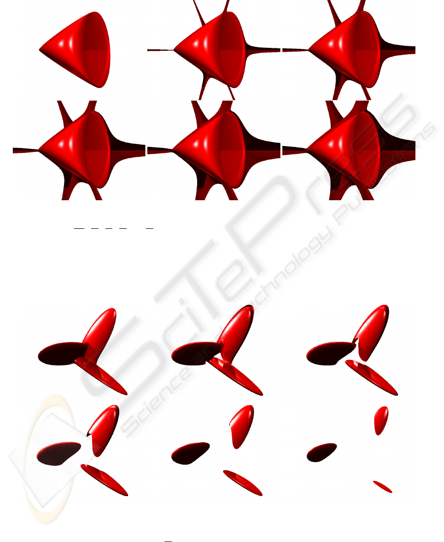
Figure 10: From up-left to down-right, Steiner surface with all real coefficients are shown, obtained using the following δ
values: 0,
π
180
,
π
90
,
π
60
,
π
45
and
π
36
. All Steiner surfaces are rendering for σ = 0.
Figure 11: From up-left to down-right, Boy surface are shown: A Boy surface with all real coefficients was rendered in real
space for σ = 0 and δ = 0 in first image. The others images show a boy surface with a complex coefficient in
complex space for σ = 0 and δ =
π
18
. The evolution of these complex coefficients was p
0
(second image), p
1
(third image), p
2
(fourth image), p
3
(fifth image) and p
4
(sixth image).
VISAPP 2006 - IMAGE FORMATION AND PROCESSING
146
