HIERARCHICAL ESTIMATION OF IMAGE FEATURES WITH

COMPENSATION OF MODEL APPROXIMATION ERRORS

Stefano Casadei

71 rue du Cardinal Lemoine, 75005 Paris, France

Keywords:

Model-based estimation, edge and corner detection, feature extraction, grouping, feedback, model hierarchy.

Abstract:

To facilitate the optimal estimation of the parameters of a complex image feature, the feature’s model is

fragmented into simpler approximating models. By repeating this fragmentation procedure recursively, a

hierarchy of feature models is obtained. To ensure that feature parameter values are recovered exactly in

the limit of high SNR, an algorithm is proposed to compensate for the model approximation errors between

adjacent levels of the hierarchy.

1 INTRODUCTION

The detection of local image features, such as edges,

corners and junctions, and the estimation of the as-

sociated parameters provide the basis for many com-

puter vision algorithms and systems. One approach

to carry out this task is to process the input image in

a feedforward way, constructing a hierarchy of fea-

tures in a bottom-up order (Marr, 1982; Nalwa and

Binford, 1986; Canny, 1986; Perona, 1995; Casadei

and Mitter, 1999a; Casadei and Mitter, 1998; Casadei

and Mitter, 1999b; Casadei and Mitter, 1996; K

othe,

2003; W

urtz and Lourens, 1997). To improve accu-

racy and to extend the applicability of the basic feed-

forward operators designed for straight-line edges,

some methods analyze the response of these operators

to more complex features, such as lines and corners

(Deriche and Giraudon, 1990; Deriche and Giraudon,

1993; Steger, 1998).

A rather different approach for feature estimation

is model-based optimization, which yields, in prin-

ciple, optimal estimates for all feature parameters.

Direct comparisions with feedforward methods have

shown the superior accuracy and detection perfor-

mance of optimization methods (Rohr, 1992; De-

riche and Blaszka, 1993; Blaszka and Deriche, 1994b;

Blaszka and Deriche, 1994a; Nayar et al., 1996;

Baker et al., 1998).

A key element of optimization methods is the use

of feedback loops to reﬁne feature parameter esti-

mates and to validate feature hypotheses. Typically,

these feedback loops are obtained by using a paramet-

ric feature model to generate image-level reconstruc-

tions of feature hypotheses and by comparing these

reconstructions with the input data.

A disadvantage of many existing model-based op-

timization methods, which are usually based on non-

linear iterative techniques such as the Levenberg-

Marquardt algorithm, is their high computational re-

quirements. Two other difﬁcult aspects of optimiza-

tion methods are parameter initialization and selec-

tion of the estimation window. These problems can be

addressed by representing complex features at multi-

ple levels of complexity and by integrating bottom-

up feedforward processing with top-down feedback

loops. By using of a hierarchy of feature models,

bootstrapping methods can be used to initialize the

parameters of complex features and more computa-

tionally efﬁcient feedback loops (based, for example,

on lookup tables) can be implemented.

The paper is organized as follows. Section 2 ex-

plains the role played by intermediate features in fa-

cilitating top-down model-based feedback and intro-

duces the key deﬁnitions underlying the proposed

methodology, which is based on fragmenting com-

plex feature models into simpler approximating mod-

els and on compensating for the model discrepancies

associated with this fragmentation (see Fig. 1). Sec-

tion 3 illustrates this general methodology with an

edge detection example where a corner model is frag-

mented into straight-line edge models. Section 4 de-

scribes a particular algorithm for model discrepancy

compensation.

381

Casadei S. (2006).

HIERARCHICAL ESTIMATION OF IMAGE FEATURES WITH COMPENSATION OF MODEL APPROXIMATION ERRORS.

In Proceedings of the First International Conference on Computer Vision Theory and Applications, pages 381-388

DOI: 10.5220/0001369003810388

 SciTePress

I = H(ϑ)+ν

−1

r(ϑ)+η

∗

H(ϑ)

˜r

−1

r(ϑ)

˜r

λ(ϑ)

Figure 1: Feature estimation with an intermediate layer of

auxiliary features. A high-level feature ϑ ∈ Θ is repre-

sented at the image level by a parametric model function

H. The same feature is represented at an intermediate level

by one or more approximating fragments, denoted λ(ϑ).

Centered estimators f for the fragments are provided which

recover the intermediate feature parameters exactly in the

limit of inﬁnite SNR. The distortion map ˜r (see (11)) de-

scribes the effect of the discrepancy (1) between the high

level feature model H and the intermediate feature models

. The right part of the diagram describes the estimation

process, which begins with an input image I containing a

feature instance plus noise ν. The noisy intermediate fea-

tures recovered by f are r(ϑ)+η. These are projected on

R  r(Θ) according to a metric based on an estimate

of ϑ (see Appendix B). The result, ϕ

∗

is then compensated

for model discrepancy by inverting the distortion map ˜r. Fi-

nally, an (updated) estimate

ϑ is obtained through λ

−1

and

a new iteration is performed.

2 INTERMEDIATE FEATURES

Parametric feature models The proposed method

for feature estimation is illustrated by the diagram in

Fig. 1, which depicts a pair of adjacent levels of a

model hierarchy and the bottom image layer. The top

layer contains the high-level feature to be estimated,

represented by a multi-dimensional feature parameter

ϑ ∈ Θ. A parametric model function, denoted H,

speciﬁes the noiseless or ideal image level represen-

tation of this high-level feature. Speciﬁcally, for any

feature parameter ϑ ∈ Θ, H(p; ϑ) denotes the noise-

less value of the feature identiﬁed by ϑ at the image

point p ∈ R

. The block of feature values associated

with a ﬁnite set of image points U ⊂ R

is denoted

H(U; ϑ). The input image is denoted I and the image

block associated with the image region U is denoted

I(U).

Model fragmentation An approach to construct a

model hierarchy is to decompose or fragment a fea-

ture instance (ϑ, U), identiﬁed by the feature para-

meter ϑ ∈ Θ and the image domain or support U ⊂

, into one or more intermediate features (ϕ

, S

k =1,...,K, having feature parameters ϕ

∈ Φ

image domains S

⊂ U, and image representations

; ϕ

), where F

are the parametric model func-

U q

b + a

b − a

Figure 2: Fragmentation of a corner feature H(U; ϑ) into

two straight-line edge features F (S

; ϕ

) and F (S

; ϕ

tions of the intermediate features. For example, a cor-

ner feature can be decomposed into two straight-line

features as described by (19), (20) and as shown in

Fig. 2.

Model fragmentation is carried out so that

; ϕ

), k =1,...,K, are local approximations

of H(U; ϑ). The associated approximation error is

referred to as model discrepancy and is denoted ∆

For any ϑ ∈ Θ, and for a particular conﬁguration of

the domains U and S

, let λ

(ϑ) ∈ Φ

be the model

parameter ϕ

chosen by the fragmentation procedure

to be the local approximator of the k-th fragment.

Then, the k-th model discrepancy is given by:

∆

(ϑ)  H(S

; ϑ) − F

; λ

(ϑ)). (1)

Generally speaking, our strategy to design accu-

rate and computationally efﬁcient feature estimators

is to construct hierarchical fragmentations of a com-

plex models into intermediate approximating models,

so that the model discrepancy between adjacent levels

of the hierarchy is sufﬁciently small to guarantee the

effectiveness and computational efﬁciency of model-

based feedback loops.

Local parametrization The functions λ

:Θ→

associated with a model fragmentation provide

a “local” parametrization for the fragmented H-

features. Indeed, model fragmentations are typically

constructed so that the joint coordinate map:

λ :Θ→ Φ  Φ

×···×Φ

(2)

given by

λ(ϑ)=(λ

(ϑ),...,λ

(ϑ)), (3)

is injective. Thus, by letting λ(Θ) ⊂ Φ be the image

of Θ under λ, which is also the set of all “consistent”

combinations of local coordinates:

λ(Θ) = {(ϕ

,...,ϕ

), ∃ϑ ∈ Θ,λ

(ϑ)=ϕ

(4)

one obtains the bijective coordinate map

λ :Θ→ λ(Θ), (5)

which yields a local reparametrization of the feature

model H.

VISAPP 2006 - IMAGE ANALYSIS

382

Feature estimators Let us assume that estimators

for the intermediate features are given and are repre-

sented by the maps:

: R

→ Φ

,k=1,...,K. (6)

That is, for a given input image I and a given image

domain S

, the estimated parameter of the interme-

diate feature is f

(I(S

)), where I(S

) is the image

block with domain S

An estimator is said to be centered if it recovers the

exact value of the feature parameter when the image

contains a noiseless instance of the feature. That is,

is centered if

; ϕ

)) = ϕ

, ∀ϕ

∈ Φ

. (7)

Note that the property of being centered is relative

to a particular feature model. For example, Canny’s

edge detector is centered only for edges with zero

curvature (see (Deriche and Giraudon, 1990; Deriche

and Giraudon, 1993; Steger, 1998) and Fig. 6). In

general, feedforward estimators are centered only for

very simple feature models. An objective of the pro-

posed method is to construct centered estimators for

complex feature models by using feedback and hier-

archical representations.

Hierarchical feedback loops In a standard, non-

hierarchical model-based approach for feature esti-

mation, a feedback loop is obtained by comparing an

input image block I(U) with the image representa-

tion H(U;

ϑ) of the current feature estimate

ϑ. The

error signal ||I(U) − H(U;

ϑ)|| and its derivatives

are used iteratively to obtain better feature estimates,

for example, through gradient descent, Gaussian-

Newton, or Levenberg-Marquardt methods.

In a model-based hierarchical approach, feedback

loops, rather than connecting directly high-level com-

plex features to their image level representations, are

mediated through one or more layers of intermediate

features. One type of feedback loop, which can be

used to compensate for model discrepancies and the

mutual interference between nearby features, is ob-

tained by comparing high-level predictions of the in-

termediate features with low-level predictions of the

same intermediate features. Speciﬁcally, the high

level predictions, denoted r

(ϑ), are obtained by ap-

plying the estimators f

, k =1,...,K to the high-

level model H(U; ϑ):

(ϑ)=f

(H(S

; ϑ)) (8)

or, more compactly,

r(ϑ)=f(H(U; ϑ)), (9)

where

f =(f

,...,f

r =(r

,...,r

(10)

and f

(H(U; ϑ)) = f

(H(S

; ϑ)).

The low-level predictions are obtained by applying

the estimators f

to the feature models F

, to yield

; λ

(ϑ))). By assuming that f

are cen-

tered estimators for the parametric models F

(or by

designing them to be so), the low-level prediction of

the k-th intermediate feature is simply λ

(ϑ) and the

joint low-level prediction is λ(ϑ). Note that to each

low-level prediction µ ∈ λ(Θ) there corresponds one

high-level prediction given by the map:

˜r : λ(Θ) → r(Θ)

˜r(µ)=f(H(U; λ

−1

(µ))).

(11)

This map describes the distortion in the intermedi-

ate feature parameter due to model discrepancy. In-

deed, notice that if all the model discrepancies ∆

(ϑ)

vanish then ˜r is the identity map.

By assuming that the map r is injective, it follows

that ˜r is bijective. Then the inverse ˜r

−1

exists and

can be used to compensate for model discrepancy, as

described in Section 4.

Parameter displacements If the space Φ in which

both λ(Θ) and r(Θ) are embedded is linear, then one

can represent the distortion map ˜r by means of the

parameter displacement map:

s(µ)  ˜r(µ) − µ, µ ∈ λ(Θ), (12)

which represents the error in predicting the intermedi-

ate features due to the discrepancy between the high-

level “integrated” model H and the elementary mod-

els F

. A more general deﬁnition (for the case where

the estimators f are not necessarily centered) is given

by:

(ϑ)  f

(H(S

; ϑ)) − f

; λ

(ϑ))). (13)

The parameter displacements can be learnt during

an ofﬂine setup stage by simulating the estimators f

on the appropriate feature instances. They can then

stored in a memory and accessed through a lookup

table during the image processing stage to compen-

sate for model discrepancies, as described in Section

4. Fig. 3 illustrates the parameter displacements due

to the discrepancy between a corner feature model and

a straight-line edge model.

3 EDGE DETECTION

3.1 A Hierarchy of Edge Models

The model hierarchy of the edge detector we have de-

veloped contains ﬁrst order (P1) and third order (P30)

polynomial models, blurred straight-line edges (SE)

HIERARCHICAL ESTIMATION OF IMAGE FEATURES WITH COMPENSATION OF MODEL APPROXIMATION

ERRORS

383

0 1 2 3

.05

0.1

.15

0.2

.25

0.3

Orientation

0 1 2 3

−0.6

−0.5

−0.4

−0.3

−0.2

−0.1

Position

0 1 2 3

0.005

0.01

0.015

0.02

0.025

0.03

Scale

0 1 2 3

−0.14

−0.12

−0.1

−0.08

−0.06

−0.04

−0.02

Stepsize

0 1 2

−0.04

−0.02

0.02

0.04

0.06

0.08

0.1

0.12

0.14

Offset

Figure 3: Parameter displacement of an SE feature due to

the discrepancy with a corner feature. The x-axis represents

the distance between the vertex of the corner point q and

the edge-line center q

of the SE feature (see Fig. 5). Each

curve is for a given value of the bending angle β, ranging

between 0 and π/2. From left to right are the displacement

of orientation and position of L

; σ, a and b. The value of

a is 1.

and corners (Co). The parametric model functions for

the three lowest levels are given by:

(p; ϑ

)=b + aX

(p), (14)

P30

(p; ϑ

P30

)=b +

(p) −

2σ

(p)

(15)

(p; ϑ

)=(b − a)+

√

2π



(p)

−∞

−





(16)

where

• ϑ

=(ψ, a, b); L

is a straight line with ori-

entation ψ orthogonal to the gradient and passing

through a reference point (e.g., the center of the

feature domain); X

(p) is the signed distance from

this line to the point p;

• ϑ

P30

=(L, a, b, σ); L is a straight line and X

(p)

is the signed distance from this line to the point p;

• ϑ

=(L, a, b, σ), where L is the edge line.

Note that H

-features are obtained by blurring step-

edge features with a gaussian ﬁlter.

To illustrate the proposed method and the deﬁni-

tions of the previous section, we focus now on the two

layers containing respectively H

-features (playing

the role of intermediate features) and H

-features

(playing the role of high-level features). A common

model for corner features is given by:

H(p; L

,a,b,σ)=b − a +2aC

(p; L

(17)

where (see Fig. 4, right panel): (L

,a,b,σ) is

the 7D parameter of corner features, henceforth de-

noted ϑ ∈ Θ; L

are oriented straight lines in

the image plane forming angles ψ

,ψ

∈ [0, 2π[,

<ψ

with a reference line; b ∈ R is the “as-

ymptotic” image value (as the distance from the cor-

ner point approaches inﬁnity) on the edge lines L

C(L

)

b − a

b + a

−L

C(−L, L)

b − a

Figure 4: Left: an SE feature with image domain S, rep-

resenting a blurred step edge with image model F (S; ϕ),

as given by (18) or, equivalently, (18). C(−L, L) is the

half-plane lying on the right of L and C(·; −L, L) is its

indicator function. Right: a corner feature with image do-

main U. The cone C(L

), whose indicator function is

C(·; L

), lies on the right of the polygonal line obtained

by connecting the lower half of −L

with the upper half of

, as shown. The function C

(·; L

) is obtained by

convolving C(·; L

) with a Gaussian ﬁlter.

and L

; 2a =0is the (signed) image value change

across the edge lines, from the left side to right side;

σ>0 is a blur parameter; C(·; L

) is the indica-

tor function of the cone C(L

) delimited by the

lines L

as shown in Fig. 4; and C

(·; L

) is

obtained by convolving C(·; L

) with a Gaussian

ﬁlter with variance σ

. To facilitate the comparison

between H

-features and H

-features, we rewrite

the former as (see Fig. 4, left panel):

F (p; L, a, b, σ)=b − a +2aC

(p; −L, L). (18)

3.2 Fragmenting Corner Features

A corner feature H(U; ϑ) is decomposed into two

blurred step-edge features F (S

; ϕ

), F (S

; ϕ

whose domains S

and S

are roughly bisected by

the two branches of the corner, as shown in Fig. 2.

For any ϑ =(L

,a,b,σ), the local parameters

(ϑ) and λ

(ϑ), which characterize the approximat-

ing straight-line edge features, are chosen as follows:

(ϑ)=(L

, −a, b, σ), (19)

(ϑ)=(L

,a,b,σ). (20)

With this choice, the discrepancies (1) between the

corner feature and the approximating straight-line

edge features vanish as the distances between S

k =1, 2 and the corner point q increases.

The parameter displacements of ϕ

can be stored in

a lookup table indexed by the parameters L

,σ,β,d,

where d is the longitudinal coordinate of the corner

point q along the line L

, as shown in Fig. 5, and β is

the deviation of the corner from a straight-line. The

values of these parameter displacements as β and d

vary while L

and σ are held ﬁx, are shown in Fig. 3.

VISAPP 2006 - IMAGE ANALYSIS

384

+ π

−L

Figure 5: The displacement of the SE parameter ϕ

(esti-

mated in the domain S

) induced by a corner feature with

vertex q and orientations ψ

, ψ

, depend on the following

variables: the edge line L

; the blur parameter σ; the signed

distance from q

to q; and the bending angle β, given by

the orientation of L

relative to −L

, and representing the

deviation of the corner’s polygonal line (−L

) from a

straight line.

3.3 Grouping Projectors

To utilize model-based feedback, it is necessary to

provide an initial estimate of the high-level model pa-

rameter ϑ. This initial estimate can be obtained from

the local parameter values ϕ =(ϕ

,...,ϕ

) ∈ Φ

calculated by the estimators f on the input image,

ϕ = f (I(U)). Formally, the operation of mapping

ϕ to an initial estimate for ϑ can be represented by an

operator

π :Φ→ λ(Θ). (21)

The initial estimate for ϑ is then λ

−1

(π(ϕ)). It will

be assumed that a local parameter ϕ that is the local

coordinate λ(ϑ

) of some high-level parameter ϑ

treated by π as such so that π is a projector from Φ to

λ(Θ):

π(µ)=µ, ∀µ ∈ λ(Θ). (22)

In our corner example, the following projector π is

used:

(ϕ

,ϕ



+ a

+ b

+ σ



(23)

where ϕ

=(L

,σ

), k =1, 2 and the signs

are chosen depending on the relative geometric

conﬁguration of L

, S

. Notice that this oper-

ator describes the basic grouping operation of form-

ing a corner feature by simply intersecting the two

straight-lines L

and L

and averaging the other pa-

rameters a

, b

, and σ

. Notice that this simple op-

eration does not yield, in general, the correct value of

the corner feature parameter ϑ in response to a noise-

less corner feature given by (17).

3.4 Estimation Algorithm

A detection algorithm that simultaneously estimates

straight-line edges and corners has been implemented

and the results of an experiment are shown in Fig.

6. The proposed method of fragmenting the feature

model and inverting the associated distortion map ˜r is

utilized twice: once to estimate SE features from P30

features and once to estimate corners from SE fea-

tures. P1 features, calculated from 2x2 image blocks,

are used to provide an initial estimate for edge ori-

entation. P30 features are calculated by least-square

ﬁtting a third order polynomial, varying only in the

direction perpedicular to the initial P1 orientation es-

timate, to all 4x4 image blocks where the P1 image

gradient is above a threshold. SE features are ob-

tained from P30 features by means of a 3D lookup

table that compensates for the SE-P30 discrepancy.

Finally, corner features are obtained by means of the

compensation method described in the next section,

applied to the corner fragmentation (19)-(20).

4 MODEL DISCREPANCY

COMPENSATION

This section describes a method to mitigate the model

discrepancies arising in a hierarchical estimation ap-

proach. Random disturbances, such as additive i.i.d.

noise, the mitigation of which is brieﬂy discussed in

Appendix B, are neglected here. Instead, note that

structured disturbances, such as those caused by the

interference of nearby features, are clearly addressed

by the method described here. Indeed, in a hierar-

chical approach, interference can be compensated for

by introducing a more global, higher level, composi-

tional model comprising the interfering elements and

modeling their mutual interference. For example, a

corner edge model describes the interference between

its two constituent straight-line edges and compen-

sating the discrepancy between corner and straight-

line features amounts to mitigating the interference

between these straight-line features.

To compensate for model discrepancy (and feature

interference) a centered estimator must be constructed

for the high-level feature parameter ϑ. If, by recur-

sion, it is assumed that centered estimators f

for the

low-level feature parameters ϕ

are available, then a

centered estimator h for ϑ can be obtained by invert-

ing the distortion map ˜r given in (11). More precisely,

let the input image be given by:

I(U)=H(U; ϑ), (24)

and let ϕ

be the intermediate feature parameters es-

timated through the estimators f:

= f(I(U)). (25)

HIERARCHICAL ESTIMATION OF IMAGE FEATURES WITH COMPENSATION OF MODEL APPROXIMATION

ERRORS

385

4 6 8 10 12 14

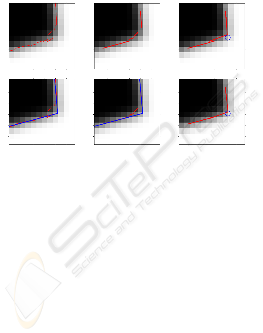
Figure 6: The results of an experiment performed with an image containing a corner feature, given by (17), with σ =1. Left

panels, with (row,column) equal to (1,1) and (2,1): result of Canny’s algorithm. The ground truth lines L

and L

are shown

in blue in the panel (2,1). Notice that Canny’s edge detector is not centered near the corner point due to the “interference”

between the straight-line edges. Center panels (1,2) and (2,2): the SE features (the ground truth lines are shown in (2,2)).

Notice that the ground truth lines cover all the SE features except for the two nearest to the corner point. Panel (1,3) shows

the result of applying the operator π, deﬁned in (23), to a pair of SE features near to the corner point. The blue circle indicates

the true position of the corner. Notice that the bottom part of the corner feature is not aligned with the SE edges. Finally,

panel (2,3) shows the edge representation after two iterations of the 0-th order compensation algorithm (32)-(33) applied to

the corner feature in panel (3,1). The bottom segment of the corner feature is now much closer to the ground truth.

Then, the estimate for ϑ given by:

ϑ = λ

−1

(˜r

−1

(ϕ

)) (26)

satisﬁes

˜r(λ(

ϑ)) = ϕ

, (27)

f(H(U;

ϑ)) = ϕ

(28)

(using (11)). Since f ◦H was assumed to be injective,

it follows that

ϑ = ϑ, so that the estimator h given by:

h(I(U)) = λ

−1

(˜r

−1

(f(I(U)))), (29)

is centered for the model function H.

Zero order algorithm By letting µ = λ(

ϑ), (26) is

equivalent to the equation

˜r(µ)=ϕ

(30)

in the unknown µ. If the map ˜r can be written in the

form (12), then (30) becomes:

µ = ϕ

− s(µ), (31)

which has a solution µ ∈ λ(Θ) if ϕ

∈ r(Θ).An

initial estimate for µ can be obtained through a pro-

jector π: µ

= π(ϕ

). This estimate can be plugged

into the right hand side of (31), to yield an updated

value µ

= ϕ

− s(µ

) which, under the 0-th order

approximation that s(µ

)  s(µ

), satisﬁes (approx-

imately) Eq. (31). If s(µ

) = s(µ

) then, in general,

− s(µ

) does not belong to λ(Θ) so that the pro-

jector π needs to be applied again. By iterating this

procedure we get

ˆµ

= π(ˆϕ

) (32)

ˆϕ

t+1

=ˆϕ

− s(ˆµ

), (33)

with initialization ˆϕ

= ϕ

. In the more general case

where ϕ

is not in r(Θ) (due to additive noise ν, see

Fig. 1) ϕ

must be projected onto r(Θ). This case is

not considered in depth here (see however Section B).

Notice that (32) represents a bottom-up “grouping”

step (compare with (23)) and (33) represents a top-

down feedback correction based on the predicted pa-

rameter displacement s(ˆµ

) (which can be precom-

puted and accessed through a lookup table). To em-

VISAPP 2006 - IMAGE ANALYSIS

386

phasize the latter point, note that (33) can be written

also as:

ˆϕ

t+1

=ˆµ



ˆϕ

− ˜r(ˆµ

)



, (34)

where ˆϕ

− ˜r(ˆµ

) is also a feedback correction.

If a ﬁxed point ˆµ of the iterative system (32)-(33)

can be found, then it yields a centered estimate for ϑ,

given by λ

−1

(ˆµ) (see Appendix A).

The results of this algorithm on a particular image

containing a corner feature are shown in Fig. 6.

First order algorithm To solve iteratively equation

(31) with a ﬁrst order approximation of the distortion

map ˜r, let us calculate its Taylor expansion from ˆµ

ˆµ

t+1

(we assume that the f

are centered):

˜r(ˆµ

t+1

)=˜r(ˆµ

R(ˆµ

) · (ˆµ

t+1

− ˆµ

), (35)

where

R(·) is the derivative matrix of ˜r(·). The equa-

tion ˜r(ˆµ

t+1

)=ϕ

, where ϕ

= f

(I(S

)), then be-

comes:

˜r(ˆµ

R(ˆµ

)(ˆµ

t+1

− ˆµ

)=ϕ

. (36)

From this, by replacing ˆµ

t+1

with ˆϕ

t+1

, we get the

iterative system:

ˆµ

= π(ˆϕ

) (37)

ˆϕ

t+1

=ˆµ

−1

(ˆµ

) ·



− ˜r(ˆµ

)



. (38)

Notice that while the 0-th order corrections (33) for

the k-th fragment depend only on the the parame-

ter displacement s

for that fragment, each ﬁrst-order

correction (38) involves the parameter displacement

of all the fragments, because the matrix

−1

is not

block diagonal in general.

5 CONCLUSIONS

Estimation of the parameters of complex features

by means of a model hierarchy, where bottom-up

bootstrapping is coupled with top-down feedback

across adjacent layers, yields better accuracy than

purely bottom-up feedforward methods, and with less

computational requirements than direct optimization

methods that do not utilize intermediate representa-

tions. A method has been described to construct

a model hierarchy by fragmenting complex features

into simpler approximating models and to carry out

parameter estimation by compensating for the asso-

ciated model approximation errors (model discrepan-

cies). When multiple fragments are present, this com-

pensating amounts to correcting the parameter distor-

tions due to the interference between the fragments.

These are some task items to be addressed by future

work: evaluate the method with more complex syn-

thetic images and with real data; compare with other

methods, such as those in (K

othe, 2003; W

urtz and

Lourens, 1997); investigate the effect of random ad-

ditive noise and develop suitable mitigation methods;

use linearization techniques to represent high dimen-

sional distortion maps as linear superpositions of low

dimensional maps, so that the method can be applied

to more complex features (e.g., N -junctions); reduce

memory requirements further by means of more so-

phisticated multidimensional interpolation methods.

ACKNOWLEDGEMENTS

Many thanks to Prof. Sanjoy Mitter for pointing out

the role of feedback and for other useful remarks and

suggestions.

A Correctness of the Algorithm

In order to prove the correctness of the algorithm

given by the iterative system (32)-(33), the following

deﬁnition is needed. Fix µ

∈ λ(Θ) and consider a

displacement δ ∈ Φ from the point µ

∈ λ(Θ) to

+ δ ∈ Φ. A displacement δ is said to be in the null

set of π at µ

, denoted δ ∈N(µ

),ifπ(µ

+δ)=µ

We say that the pair (π, f) discriminates the feature

model H if the displacement between the responses

of f to a pair of H-features with local coordinates

,µ

is never in the null set of π at µ

, that is, if for

any µ

,µ

∈ λ(Θ):

= µ

⇒ ˜r(µ

) − ˜r(µ

) ∈N(µ

Proposition. If f

is centered for all k =

1,...,K; (π, f) discriminates the feature model H;

and the system (32)-(33) always converges, then the

resulting estimator is centered for the feature model

Proof. We can assume:

I(S

)=H(S

; ϑ),

for some ϑ ∈ Θ, so that

ˆϕ

= f

(H(S

; ϑ)) = ˜r

(µ), (39)

where µ = λ(ϑ). First, let us show that µ is a ﬁxed

point, that is, ˆϕ

=ˆϕ

t+1

=ˆµ

= µ satisﬁes both

(32) and (33). (32) is clearly satisﬁed because π is a

projector on λ(Φ) (see (22)). As for (33), we need to

show that the right hand side is equal to µ. Indeed, by

using (12) and (39) we have:

ˆϕ

− s

(µ)=˜r

(µ) − ˜r

(µ)+µ

= µ

Now, let us show that µ is the only ﬁxed point. If ˆµ

is a ﬁxed point then, for some ˆϕ ∈ Φ,

ˆµ = π(ˆϕ) (40)

ˆϕ =˜r(µ) − ˜r(ˆµ)+ˆµ. (41)

HIERARCHICAL ESTIMATION OF IMAGE FEATURES WITH COMPENSATION OF MODEL APPROXIMATION

ERRORS

387

From (40) we have that ˆϕ − ˆµ is a null displacement

for π at ˆµ: ˆϕ − ˆµ ∈N(ˆµ); combining this with (41):

˜r(µ) − ˜r(ˆµ)= ˆϕ − ˆµ ∈N(ˆµ). Since (π, f) discrim-

inates the feature model H, this implies ˆµ = µ.

B Mitigation of Additive iid Noise

If the image contains an H-feature instance corrupted

by unstructured noise, that is,

I(U)=H(U; ϑ)+ν (42)

where ν represents a block of identically indepen-

dently distributed random variables, then the estima-

tors f

, when applied to the input image I, yield the

intermediate feature ϕ ∈ Φ given by:

ϕ = f (I(U)) = f(H(U; ϑ)+ν)=r(ϑ)+η, (43)

where η is a random variable. If f can be linearized:

ϕ  f (H(ϑ)) + ∇f (H(ϑ)) · ν, (44)

where, for notational simplicity, we let f (H(ϑ)) ≡

f(H(U; ϑ)), then the covariance of ϕ, conditional on

the image containing an H-feature with model para-

meter ϑ, is:

(ϑ)=(∇f(H(ϑ)))



· Σ

iid

·∇f(H(ϑ)), (45)

where Σ

iid

= σ

1 is the covariance of ν. If an esti-

mate of ϑ is available, denoted

ϑ, then ϕ can be pro-

jected to r(Θ) based on the metric Σ

(ϑ) given by

(45), which amounts to a maximum-likelihood (ML)

ﬁltering of the noise signals ν and η, to yield

∗

= π

(ϕ), (46)

where π

R|ϑ

denotes the projector from Φ to R 

r(Θ) based on the metric Σ

(ϑ).

REFERENCES

Baker, S., Nayar, S., and Murase, H. (1998). Parametric

feature detection. IJCV, 27:27–50.

Blaszka, T. and Deriche, R. (1994a). A model based method

for characterization and location of curved image fea-

tures. Technical Report 2451, Inria-Sophia.

Blaszka, T. and Deriche, R. (1994b). Recovering and

characterizing image features using an efﬁcient model

based approach. Technical Report 2422, INRIA.

Canny, J. (1986). A computational approach to edge detec-

tion. PAMI, 8:679–698.

Casadei, S. and Mitter, S. K. (1996). A hierarchical ap-

proach to high resolution edge contour reconstruction.

In CVPR, pages 149–153.

Casadei, S. and Mitter, S. K. (1998). Hierarchical image

segmentation – part i: Detection of regular curves in a

vector graph. IJCV, 27(3):71–100.

Casadei, S. and Mitter, S. K. (1999a). Beyond the unique-

ness assumption : ambiguity representation and re-

dundancy elimination in the computation of a cover-

ing sample of salient contour cycles. Computer Vision

and Image Understanding.

Casadei, S. and Mitter, S. K. (1999b). An efﬁcient and prov-

ably correct algorithm for the multiscale estimation of

image contours by means of polygonal lines. IEEE

Trans. Information Theory, 45(3).

Deriche, R. and Blaszka, T. (1993). Recovering and charac-

terizing image features using an efﬁcient model based

approach. In CVPR.

Deriche, R. and Giraudon, G. (1990). Accurate corner de-

tection: An analytical study. ICCV, 90:66–70.

Deriche, R. and Giraudon, G. (1993). A computational

approach for corner and vertex detection. IJCV,

10(2):101–124.

othe, U. (2003). Integrated edge and junction detection

with the boundary tensor. In ICCV ’03, page 424.

Marr, D. (1982). Vision. W.H.Freeman & Co.

Nalwa, V. S. and Binford, T. O. (1986). On detecting edges.

PAMI, 8:699–714.

Nayar, S., Baker, S., and Murase, H. (1996). Parametric

feature detection. In CVPR, pages 471–477.

Perona, P. (1995). Deformable kernels for early vision.

PAMI, 17:488–499.

Rohr, K. (1992). Recognizing corners by ﬁtting parametric

models. IJCV, 9(3).

Steger, C. (1998). An unbiased detector of curvilinear struc-

tures. PAMI, 20(2):113–125.

urtz, R. P. and Lourens, T. (1997). Corner detection

in color images by multiscale combination of end-

stopped cortical cells. In ICANN ’97: Proceedings of

the 7th International Conference on Artiﬁcial Neural

Networks, pages 901–906, London, UK. Springer-

Verlag.

VISAPP 2006 - IMAGE ANALYSIS

388