
STRATEGIES FOR FAST TRUE MOTION BLOCK MATCHING
Hendrik van der Heijden, Fabian Wenzel, Rolf-Rainer Grigat
Hamburg University of Technology
Vision Systems, 4-08/1
Harburger Schlossstr. 20
21079 Hamburg, Germany
Keywords:
fast block matching, motion estimation, true motion.
Abstract:
Block matching is a widely used method for fast motion estimation. Although using a very simple motion
model, which does not fit most real world video material, many motion compensating video compression
algorithms use block matching because of its speed. Applications based on true motion vector estimates often
use an optical flow algorithm because of their higher need for accuracy at the expense of increased computing
time. This paper presents a modified block matching algorithm suitable for true motion applications. A
modified full search will be used on a cost function consisting of SAD and a vector field smoothing term.
Several strategies as search center prediction, spiral search, early search termination and multilevel successive
elimination are implemented to keep the computational demand low. This way, high-quality estimates can be
computed in real-time.
1 INTRODUCTION
Motion Estimation (ME) is the basis for many digital
image processing applications. In video coding, the
objective of a ME algorithm is to minimize the resid-
ual intensity difference after motion compensation.
Mostly block matching ME algorithms are used here
because of speed. Typically, ME through minimiz-
ing intensity differences is not identical to determin-
ing true motion, which is defined as the physical 3D
motion projected onto the image plane. If true motion
estimates are required, ME is usually done by an op-
tical flow (OF) algorithm, which tend to be time con-
suming. This paper adopts a motion smoothness con-
straint, as it is an essential aspect of optical flow algo-
rithms, to be used in block matching. As search space
subsampling algorithms like three step search are not
suitable for true motion estimation, an adapted full
search is used. Several techniques are implemented
to keep computational demands low on today’s desk-
top PCs. While the resulting motion field still has
block resolution, correctness of estimates may im-
prove from this added constraint, making it useful
for some applications which otherwise would need a
computational intensive optical flow approach.
2 BLOCK MATCHING
Block matching algorithms calculate a motion vector
field, which consists of one vector for each block in
the current frame pointing to its correspondence in a
reference frame. The current frame I
t
is divided into
non-overlapping square blocks of size B × B, typi-
cally 16 × 16 pixels. For each block B
i,j
at position
(x, y) a corresponding block of the same size at posi-
tion (x + v
x
,y + v
y
) in the reference image I
t+1
is
determined by solving the following equation:
v =(v
x
,v
y
) = argmin
(v
x
,v
y
)∈S
C
(x,y )
(v
x
,v
y
) (1)
Hence, a matching error C
(x,y )
is minimized over
a set S of search positions. The resulting displace-
ment vector v is assumed to represent the motion of
the block. Typically, a cost function like the sum of
absolute differences (SAD) is chosen.
SAD
(x,y )
(v
x
,v
y
)=
B−1
j=0
B−1
i=0
|I
t
(x + i, y + j) − I
t+1
(x + v
x
+ i, y + v
y
+ j)|
(2)
359
van der Heijden H., Wenzel F. and Grigat R. (2006).
STRATEGIES FOR FAST TRUE MOTION BLOCK MATCHING.
In Proceedings of the First International Conference on Computer Vision Theory and Applications, pages 359-363
DOI: 10.5220/0001368503590363
Copyright
c
SciTePress

2.1 Construction of the Search Space
The search space S is a set of discrete search positions
with integer coordinates, as the SAD function defines
no finer resolution. A full search defines S as the set
containing every position within a rectangle with size
2sw +1(sw: search window size).
S = {(v
x
,v
y
)|−sw ≤ v
x
,v
y
≤ sw} (3)
Other algorithms like Three Step Search (Wang and
Mersereau, 1999) or 2D Logarithmic Search (Jain and
Jain, 1981) reduce the number of initial search posi-
tions to 9 resp. 5 and add more positions near the min-
imum position in several steps. As, due to their con-
struction, a best match is not guaranteed to be found,
only full search is used in the following.
Solving (1) is done by evaluating the SAD for
every position in S. The SAD calculation can be
aborted early, if the partial SAD already is above the
lowest SAD found so far.
Further speedup is possible by reducing the number
of search positions (early abort of search), the com-
plexity of SAD calculation (using estimates for the
SAD) and optimizing the visiting order of the search
positions. All of these possibilities are used in this
work and described in the following sections.
2.2 Multilevel Successive
Elimination Algorithm
The Multilevel Successive Elimination Algorithm
(MSEA) (Gao, 2003) speeds up SAD calculation.
It defines several lower bounds SAD
l
on the SAD
with decreasing quality and computational demands
to speed up SAD calculation.
Consider P
0
as the set of all pixel positions in
a block. P
l,i
is the level-l quad-tree partition i of
P
0
, it contains all pixels of sub-block i with size
B
2
l
×
B
2
l
. Vectors a and b contain all pixels of the
two blocks to be compared. The evaluation of a new
search position consists of subsequently computing
SAD
L
, SAD
L−1
... SAD
0
, and is aborted as soon
as SAD
l
>SAD
∗
, SAD
∗
being the lowest SAD
found so far.
SAD ≤ SAD
l
=
0≤j≤l
i∈P
l,j
a
i
−
i∈P
l,j
b
i
(4)
The sums over block partitions are precalculated
for every position in the reference image I
t+1
and
every level, taking additional memory of 2(L +1)
times the size of a single input image. Precalculation
time for B=16 and 2 levels equals that of 4.5 SAD
calculations per block. In this case, most positions
with sub-optimal SAD values can be eliminated with
1
16
of the operations a regular SAD would take.
2.3 Prediction and Search Position
Order
It can be seen in section 2.2 that MSEA performes
well if a good search position is known as early as
possible. This fact can be utilized as neighboring
blocks tend to have highly correlated motion vectors
(MVs). In our approach MVs of three adjacent blocks
(left, top and top-right, which have already been com-
puted), three temporally adjacent block MV (same
block, bottom-left and bottom-right in the previous
motion field) and the zero motion MV are evaluated
first. This choice of neighbors is taken from (Tourapis
et al., 2001) and extended by the two diagonal tempo-
ral candidates from (de Haan et al., 1993) to allow
better prediction of upward motion.
The MV having the lowest SAD defines the search
center. As this prediction most of the time leads to the
global minimum SAD being near the search center,
the remaining positions of S are visited in expanding
spiral order starting from the search center. The ef-
fective size of the search window will be larger than
that of a static search center, because the search win-
dow size now limits the maximum detectable accel-
eration instead of the maximum speed. The search is
aborted, if n rings have been completed without find-
ing a lower cost position. n can be adjusted to favor
speed or quality of the algorithm. In the following
experiments n =3is used.
2.4 Modification Towards True
Motion
Optical flow algorithms often incorporate a motion
field smoothness constraint so that local variations in-
crease cost (Brox et al., 2004). Equations determining
MVs usually include image intensities of just a few
pixels directly, which barely is a sound measure of im-
age part similarity, even in strongly textured regions.
Constraining adjacent MVs to be similar adds indi-
rect influence of more pixels, expanding the effective
image area used for similarity measurement, which
lowers noise sensitivity. As a second effect, uniform
image regions adopt MVs of surrounding textured re-
gions.
While block matching directly includes enough
pixels for textured regions, the SAD measure is not
meaningful in poorly textured regions, regions with
non-zero gradient in only one direction or when cal-
culated on periodic image content. In this cases, tak-
ing adjacent MVs into account may improve correct-
ness of determined motion vectors. In our work, we
combine the SAD with an additive term increasing
with MV distance from its surrounding MVs, leading
to a modified cost function (5).
VISAPP 2006 - MOTION, TRACKING AND STEREO VISION
360
C(u, v)=SAD(u, v)+dB
2
f(min
i
(u, v) − N
i
)
(5)
f(x)=
x
2
if x ≤ 1
x else
(6)
N
i
are the left, top and top-right neighbor block
MVs, the distance to the nearest MV is embedded in
a function f which reduces damping for small (sub-
pixel) deviations. As only the distance to the nearest
MV is considered, the damping term penalizes posi-
tions which do not have at least one similar neighbor
MV. A neighbour MV reliability based weighting of
influence would be preferable, but was not considered
here. Damping factor d can be adjusted to the proper-
ties of the input images. In our experiments d =0.5
is a good value for most cases with B =16.
2.5 Subpixel Resolution
After determining the best matching pixel position for
a block, a second search is done around this location
refining the MV to subpixel resolution. A 2D loga-
rithmic search with an initial search distance of 1/2
pixel evaluates the cost function on the current block
and a linearly interpolated block from the reference
image. MSEA is only applicable at full-pixel posi-
tions, so subpixel refinement can take more time than
all other ME components together.
2.6 Motion Field Upsampling
In order to provide motion vectors for every pixel
in an image, the block-based vector field is upsam-
pled with one of three algorithms: constant and lin-
ear interpolation as well as hierarchical block ero-
sion(de Haan et al., 1993). The latter divides each
block in four sub-blocks and assigns the vector me-
dian of its parents vector and the vectors of its two
directly adjacent blocks of parent size to each sub-
block. This filter is applied iteratively down to sub-
blocks of size 2 ×2 pixels, then constant interpolation
is applied to save time.
3 EVALUATION
We evaluated our proposed algorithm with respect to
computing time (on an Athlon64 3000+) and accu-
racy. In order to evaluate the true error, the synthetic
yosemite sequence (Quam, 1984) with known cor-
rect motion field (ground truth) has been used. A
simple 3 × 3 smoothing filter kernel is applied to
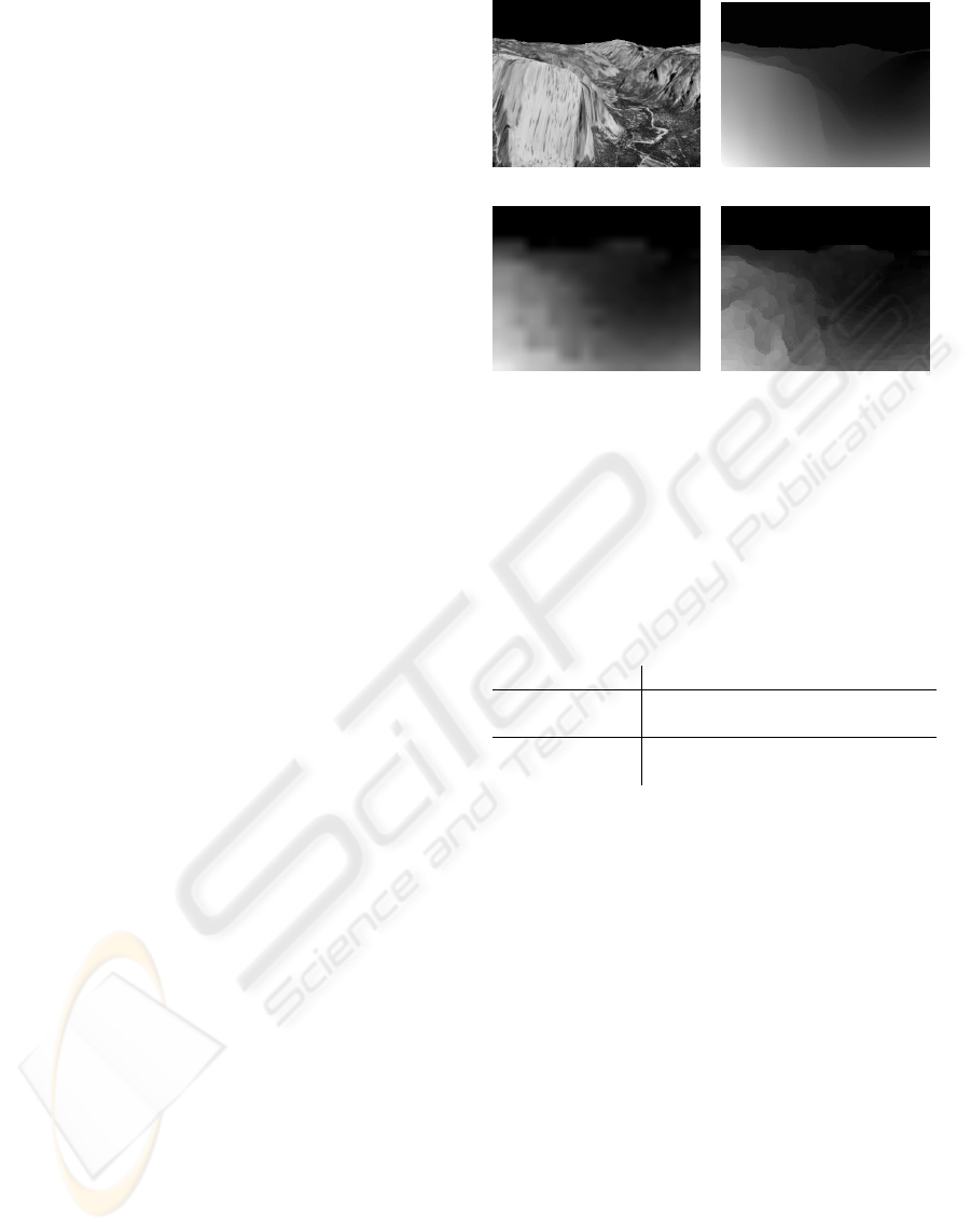
decrease aliasing effects. Figure 1 shows a sample
frame, ground truth and motion estimates.
(a) Frame 2 (b) Ground truth
(c) estimate, linear inter-
polation, B=16
(d) estimate, block ero-
sion, B=8
Figure 1: Yosemite sequence, velocity fields of correct mo-
tion (ground truth) and two estimates.
Table 1: AAE improvement when using our smoothness
constraint. For d =0, our cost function degrades to stan-
dard SAD. Other parameters are B =16, sw =16,
1/32 pixel MV resolution, linear interpolation. Computa-
tion times are given for the whole sequence.
Sequence d AAE time
Yosemite with 0 3.84
◦
± 6.91
◦
399ms
black sky
0.71 3.43
◦
± 5.71
◦
389ms
Yosemite with 0 2.80
◦
± 3.72
◦
328ms
sky cropped
0.5 2.52
◦
± 2.19
◦
351ms
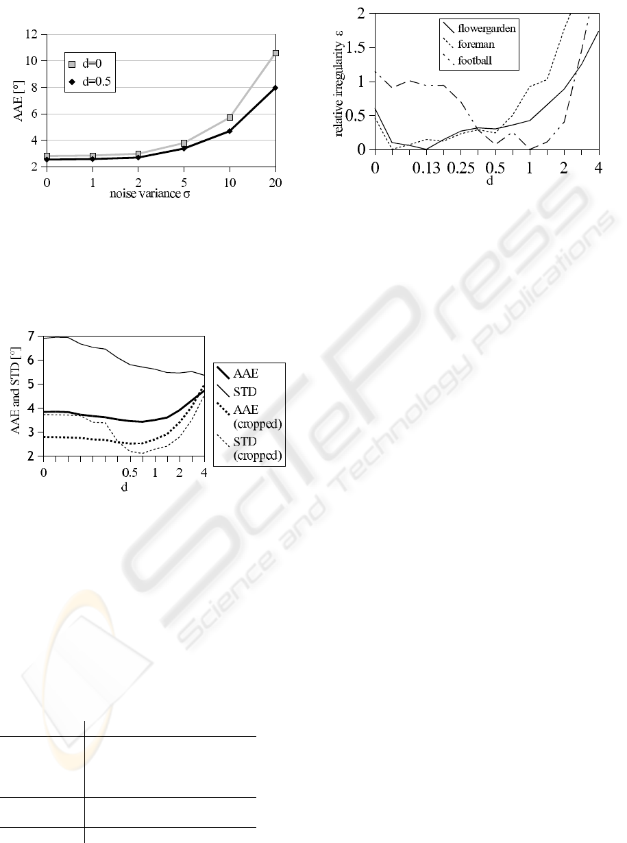
Figure 3 displays the average angular error (Horn
and Schunck, 1981) and its standard deviation at dif-
ferent damping factors. As the boundary between sky
and land cannot be modeled adequately with blocks,
a second measurement is taken with the top 72 pixel
lines cropped. Results of these tests in table 3.1 show
slight improvements of angular error and standard de-
viation when using our motion field smoothness con-
straint. While computation gets a bit faster due to
the large black area in the first test, our extension in-
creases computation time by 7% in the second test.
3.1 Noise Sensitivity
To evaluate noise sensitivity in textured regions,
we added gaussian noise with variance σ ∈
[0, 1, 2, 5, 10, 20] to the Yosemite sequence with
cropped sky and measured the AAE with and with-
out our damping extension. Results in figure 2 shows
some improvement in noisy cases.
STRATEGIES FOR FAST TRUE MOTION BLOCK MATCHING
361
(a) Frame 2
Figure 2: Noise sensitivity, average angular error of motion
estimates on Yosemite sequence (sky cropped) with added
gaussian noise.
Figure 3: Yosemite sequence, average angular error (AAE)
and standard deviation (STD) of full image with black sky
and with sky cropped at different damping factors, B=16,
upsampling via linear interpolation. Minimum values are
3.43 ± 5.71 (full) resp. 2.53 ± 2.11 (cropped).
Table 2: Yosemite sequence, linear interpolation, B =16,
sw =16, d =0.71 (optimal). For a block size of B =8
two additional results are given. For comparison, a good
100% density 2D OF result (Farneb
¨
ack, 2000) is listed, its
computing time is 16s per frame on a 360MHz Sun Ultra
60.
resolution AAE time/frame
1 pixel 8.94
◦
± 8.94
◦
11.9ms
1/2
5.02
◦
± 6.08
◦
14.7ms
1/8
3.55
◦
± 5.73
◦
23.0ms
1/32
3.43
◦
± 5.71
◦
32.6ms
1 (BS=8) 9.10
◦
± 9.35
◦
24.9ms
1/32 (BS=8)
3.54
◦
± 5.31
◦
53.7ms
OF 1.40
◦
± 2.57
◦
see caption
Figure 4: Relative irregularity at different damping factors,
minimum set to zero, block erosion, B=16.
3.2 Real World Sequences
In a second experiment, real world sequences with un-
known ground truth, a motion field irregularity mea-
sure ε (7) is used, which is defined as the average an-
gular error (AAE) between a forward ME to the next
image and a backward ME to the previous image.
ε(I
t
)=AAE(−BM(I
t
,I
t+1
),BM(I
t
,I
t−1
)) (7)
This measure yields low values when computed
correspondences are stable. False correspondences
result in motion vectors jumping from one frame to
another, i.e. in large values of . Experiments with
various parameters on several synthetic image se-
quences indicate an approximately linear connection
between ε and ground truth AAE.
Figure 4 shows the irregularity of three stan-
dard sequences, flowergarden (uniform fore-
gound/background motion), foreman (first 70 frames
only, medium motion) and football (fast, turbulent
motion).
3.3 Computation Time
Table 3 gives computation times for three standard se-
quences for pixel resolution and the additional time
per subpixel bit, which has shown to be nearly con-
stant independent of subpixel resolution, for block
sizes B =8and B =16. The impact of MSEA
on computation time was also measured in a short ex-
periment. While a spiral full search speeds up by a
factor of two, our described search algorithm gains
only about 10% speed for d =0and loses up to 4%
with d =0.5 in the flowergarden sequence. In the lat-
ter case, the overhead introduced by MSEA is larger
than the time it saves. MSEA gives best speedup on
sequences with poor motion predictabiliy, which usu-
ally are one taking the most time.
VISAPP 2006 - MOTION, TRACKING AND STEREO VISION
362

Table 3: Computing times per frame for three sequences
(block erosion, sw=16, d=0.5).
block sequence time for additional time
size
pixel res. per subpixel bit
flowergarden 29.1ms 7.6ms
8
foreman 31.3ms 8.3ms
football 33.1ms 8.3ms
flowergarden 14.4ms 5.5ms
16
foreman 16.6ms 6.6ms
football 19.8ms 6.7ms
As can be calculated from table table 3, CIF
(352x288) sized image sequences can be processed
in real time (25Hz, below 40ms per frame) with 1/8
pixel resolution, even when containing turbulent mo-
tion like in the football sequence. As processing time
is data dependent, subpixel resolution or the early ter-
mination criterion can be adaptively adjusted to meet
real time requirements for every frame. Only one vec-
tor per block is computed, so our results have lower
resolution than optical flow estimates. On compara-
ble hardware, a recent OF implementation (Bruhn and
Weickert, 2005) takes about 150ms per 160x120 pixel
frame.
4 CONCLUSION
We presented strategies for fast true motion block
matching. Our damping extension improves block
matching results towards optical flow estimation and
reduces noise sensibility. Block erosion upscaling
of motion estimates to pixel resolution removes vis-
ible block structure. Prediction and MSEA have been
adopted to keep computational demands low enough
for real time processing. As motion discontinuities
are rather badly modeled by the block structure used,
there is a desire for better edge treatment. This can
be done in several ways, for example weighting the
SAD cost with a windowing function and finding cor-
respondences for overlapping blocks as in the exper-
imental BBC Dirac video codec. Another approach
would be recognizing blocks containing more than
one motion domain and determining a decomposi-
tion of block content and motion vectors with mini-
mal SAD for each part (Orchard, 1993).
REFERENCES
Brox, T., Bruhn, A., Papenberg, N., and Weickert, J. (2004).
High accuracy optical flow estimation based on a the-
ory for warping. In Proceedings of the 8th European
Conference on Computer Vision.
Bruhn, A. and Weickert, J. (2005). Towards ultimate motion
estimation: Combining highest accuracy with real-
time performance. To appear in Proc. 10th Interna-
tional Conference on Computer Vision (ICCV 2005).
de Haan, G., Biezen, P., Huijgen, H., and Ojo, O.
(1993). True-motion estimation with 3d recursive
search block matching. IEEE Trans. on Circuits and
Systems for Video Tech., 3(5).
Farneb
¨
ack, G. (2000). Fast and accurate motion estima-
tion using orientation tensors and parametric motion
models. In Proceedings of 15th IAPR International
Conference on Pattern Recognition, September 2000.
Gao, Duanmu, Z. (2003). A multilevel successive elimina-
tion algorithm for block matching motion estimation.
IEEE Trans. on Image Processing, 9(3).
Horn, B. and Schunck, B. (1981). Determining optical flow.
Artificial Intelligence, 17(1-3):185–203.
Jain, J. and Jain, A. (1981). Displacement measurement
and its application in interframe image coding. IEEE
Trans. Commun., COM-29:1799–1808.
Orchard, M. (1993). Predictive motion-field segmentation
for image sequence coding. IEEE Trans. on Circuits
and Systems for Video Tech., 3:54–70.
Quam, L. (1984). Yosemite image sequence.
Tourapis, A. M., Au, O. C., and Liou, M. L. (2001). Pre-
dictive motion vector field adaptive search technique
(PMVFAST) - enhancing block based motion estima-
tion. In Proceedings of Visual Communications and
Image Processing 2001 (VCIP’01).
Wang, H. and Mersereau, R. (1999). Fast algorithms for the
estimation of motion vectors. IEEE Transactions on
Image Processing, 8(3).
STRATEGIES FOR FAST TRUE MOTION BLOCK MATCHING
363
