
REGISTRATION OF 3D - PATTERNS AND SHAPES WITH
CHARACTERISTIC POINTS
Darko Dimitrov, Christian Knauer and Klaus Kriegel
Freie Universit
¨
at Berlin, Institute of Computer Science
Takustrasse 9, D-14195 Berlin, Germany
Keywords:
Computational Geometry, Pattern Matching, 3D Image Registration.
Abstract:
We study approximation algorithms for a matching problem that is motivated by medical applications. Given
a small set of points P ⊂ R
3
and a surface S, the optimal matching of P with S is represented by a rigid
transformation which maps P as ‘close as possible’ to S. Previous solutions either require polynomial runtime
of high degree or they make use of heuristic techniques which could be trapped in some local minimum.
We propose a modification of the problem setting by introducing small subsets of so called characteristic
points P
c
⊆ P and S
c
⊆ S, and assuming that points from P
c
must be matched with points from S
c
.
We focus our attention on the first nontrivial case that occurs if |P
c
| =2, and show that this restriction
results in new fast and reliable algorithms for the matching problem. In contrast to heuristic approaches our
algorithm provides guarantees on the approximation factor of the matching. Experimental results are provided
for surfaces reconstructed from real and synthetic data.
1 MOTIVATION AND RELATED
WORK
Today an increasing number of surgeries is supported
by medical navigation systems. The basic task of such
a system is to transform real world data (positions in
the operating field) into a 3-dimensional model (CT
or MR) and to display the transformed position in the
model. Real world data are gaged by optical, elec-
tromagnetic or mechanical tracking systems. A com-
mon technique for computing the transformation is
based on markers which are fixed on bones (land-
mark approach). The markers have to be fixed al-
ready during the model acquisition. Their positions
in the model are computed using appropriate image
processing methods. Later, at the beginning of the
surgery, at least three markers must be gaged with the
tracking system. Since the total number of markers is
small, one could compute the correct matching trans-
formation even by brute force techniques. A more
advanced approach making use of geometric hashing
techniques is presented in (Hoffmann et al., 1999).
There is a strong need to develop algorithmic meth-
ods for computing a transformation without using
markers. The main reason for that is an anatomical
one: in many cases (e.g. spinal surgery) it would be
very hard or even impossible to fix markers before the
surgery. One solution is to gage a few points on the
surface of a bone and to compute the corresponding
points in the model. This point registration is a hard
algorithmic problem, which cannot be solved by the
following standard approaches:
1) A combinatorial search does not work, because the
gaged points could be anywhere on the model surface.
2) Surface matching algorithms do not help, because
the number of gaged points is too small to apply a
surface reconstruction.
There are heuristic methods that could be used,
for example a combination of ICP (Iterative Closest
Point) method with randomly generated starting con-
figurations. The standard ICP approach, and several
more efficient variants and generalizations of it can
be found in (Besl and McKay, 1992), (Rusinkiewicz
and Levoy, 2001), and (Mitra et al., 2004). However
such heuristic methods have the fundamental draw-
back that they could be trapped in some local mini-
mum, while failing to find the optimal solution. In
contrast to this, we will present a registration algo-
rithm that reports all possible registration transforma-
tions satisfying a given quality criterion. This is an
essential property, especially in medical applications.
Matching problems have been studied intensively
393
Dimitrov D., Knauer C. and Kriegel K. (2006).
REGISTRATION OF 3D - PATTERNS AND SHAPES WITH CHARACTERISTIC POINTS.
In Proceedings of the First International Conference on Computer Vision Theory and Applications, pages 393-400
DOI: 10.5220/0001368303930400
Copyright
c
SciTePress

in computational geometry, see (Alt and Guibas,
1999) for an overview. Nevertheless the best known
approaches applicable to our problem require poly-
nomial runtime of high degree (Hagedoorn, 2000).
Since the registration is part of the surgery, real time
algorithms are needed. In contrast to that, it is possi-
ble to spend more time for preprocessing the model.
Here, we try to adapt some ideas of the landmark
approach to that new setting. The role of markers is
played by so-called characteristic points. Such points
can be determined automatically (see next two para-
graphs) or manually, marking some anatomically sig-
nificant points, e.g. the thorn of a vertebra or the root
of the nose. If a set of characteristic points is fixed in
the model and we can track at least three of them, the
old landmark registration algorithms can be applied.
Our main goal is to solve the registration problem if
only two characteristic points can be tracked. To com-
pute the transformation in that case, one must track
some more (non-characteristic) points on the surface.
Different approaches can be applied to find char-
acteristic points on the sampled surface. A lot of ef-
fort was devoted on determining the curvature esti-
mation. A comprehensive survey of these methods is
given in (Petitjean, 2002). Popular methods include
quadric fitting, where the estimated curvature is the
one of the quadric that best fits the sampled point lo-
cally. Other methods typically consider some defin-
ition of curvature that can be extended to the poly-
hedral setting. Estimating the curvature by a canoni-
cal mapping between the mesh describing the object
and a standard spherical mesh was done in (Delingette
et al., 1993). More examples of estimating the dis-
crete curvature can be found in (Zhang, 1999), and
(Kim et al., 1999). The definition of the curvature
tensor in (Cohen-Steiner and Morvan, 2003) is based
on the theory of normal cycles.
Sometimes technics to characterize points of the
surface are strongly related with surface matching
heuristics, e.g. the spin image approach in (Johnson
and Hebert, 1997), surface point signatures in (Ya-
many and Farag, 2002), harmonic shape images in
(Zhang and Hebert, 1999), and fingerprints (Sun and
Abidi, 2001). A method described in (Wang et al.,
2000) is based on geodesic distances in combination
with additional local curvature parameters.
In this paper we present a new geometric approach
to the matching problem with characteristic points.
Some preliminary ideas were already presented in
the form of an extended abstract in (Dimitrov et al.,
2005). In the next section we introduce necessary no-
tations and give a formal definition of the problem.
In section 3 we present the basic algorithm and show
how to use this method for the approximation of the
optimal matching. Experimental results on real and
synthetic data are provided in section 4, and conclu-
sions and future work are given in section 5.
2 FORMAL PROBLEM
DESCRIPTION
We consider two point sets P and S in R
3
. Usually
we assume that S is the (infinite) set of points on a
triangulated surface. The corresponding triangulation
will be denoted by S. However, this assumption is
not crucial. The algorithms presented in the next sec-
tions can be applied with small changes if S is a finite,
dense sample of points on a surface.
Our main goal is to register P into a model S. The
quality of the registration will be evaluated by the di-
rected Hausdorff distance. The distance between a
point a and a compact point set B in d-dimensional
space R
d
is defined as
dist(a, B) = min
b∈B
||a − b||
where ||·||is the Euclidean norm in R
d
. For two com-
pact sets A, B in the one-sided Hausdorff distance
from A to B is defined as
−→
H(A, B) = max
a∈A
dist(a, B) = max
a∈A
min
b∈B
||a − b||.
The size of a problem instance (P, S) depends on
two parameters: k, the number of points in P, and n,
the number of triangles in S. We remark that in our
applications k<<ncan be assumed. Moreover, we
assume that two subsets of characteristic points S
c
⊆
S and P
c
⊆ P are given. For a precise analysis of
our algorithms we introduce the additional parameters
k
c
= |P
c
| and n
c
= |S
c
|. Both parameters should be
seen as some reasonable constants. The special role
of characteristic points is expressed by the additional
requirement, that each p ∈ P
c
must be mapped onto
(or close to) a characteristic point q ∈ S
c
.
First we have to classify several types of matchings.
Definition 2.1 Given two parameters µ, η ≥ 0 a
rigid transformation T : R
3
→ R
3
is called (µ, η)-
matching if the following two conditions hold:
1. µ(T ):=
−→
H (T (P \ P
c
),S) ≤ µ, and
2. η(T ):=
−→
H(T (P
c
),S
c
) ≤ η.
If is an upper bound for µ(T ) and η(T ) we de-
note T as an -matching. In line with the notations
above, we define (T ) = max(µ(T ),η(T )). The
minimal (T ) over all rigid transformations T is de-
noted by
opt
, and a corresponding matching is an op-
timal matching. For a given λ>1, a matching T is a
λ-approximate matching,if(T ) ≤ λ
opt
.
Furthermore, we introduce the notion of semi-
optimal matchings. To this end we fix a se-
quence
S =(¯s
1
, ¯s
2
,...,¯s
k
c
) of predefined match-
ing positions for the sequence of characteristic points
(p
1
,p
2
,...,p
k
c
). We restrict our attention to match-
ings T with T (p
i
)=¯s
i
for i =1,...,k
c
. Let us
VISAPP 2006 - IMAGE ANALYSIS
394

denote this set of matchings by M
S
. We assume that
P
c
and S are congruent, because otherwise M
S
is
empty.
A matching T ∈M
S
is a (µ(T ),η
0
)-matching,
where η
0
=
−→
H (S,S
c
) is a common value for all
matchings in M
S
. A matching T ∈M
S
is called
semioptimal matching (with respect to
S)ifµ(T ) is
minimal.
A trivial case with |M
S
| =1occurs, if P
c
contains
three or more non-collinear points. Thus, we will fo-
cus our attention to matchings with two characteristic
points. In a first step we design an algorithm to com-
pute semioptimal matchings for a given set
S. Then,
based on the semioptimal solution, we show how to
compute a λ-approximate matching for any λ>1.
3 THE 2 POINT CASE
3.1 Semioptimal Matchings
In general a rigid transformation in 3-dimensional
space has six degrees of freedom: three for fixing a
translation and three more describing a rotation. The
first step of our approach is devoted to a very special
case with one degree of freedom only. Assuming a
pair
S =(s
1
, s
2
) of predefined matching positions
for the two characteristic points p
1
,p
2
, the matchings
in T ∈M
S
have a fixed translation (T (p
1
)=s
1
)
and two fixed parameters of the rotation (mapping the
axis (p
1
,p
2
) to the axis (s
1
, s
2
)). Thus, it remains to
consider all rotations around the axis (
s
1
, s
2
). First,
we present an algorithm which reports (for any µ) all
transformations T ∈M
S
with µ(T ) ≤ µ.
Basic Algorithm (Outline)
1. Fix a rigid transformation T
0
: R
3
→ R
3
such that T
0
(p
1
)=s
1
,T
0
(p
2
)=s
2
. For all
p
i
∈ P \{p
1
,p
2
} let C
i
= C(p
i
) be the circle with
the following properties (see figure 1):
• the center of C
i
is on the line defined by p
1
and
p
2
,
• C
i
lies in a plane perpendicular to p
1
,p
2
, and
• p
i
is on C
i
.
2. Consider the transformed circle T
0
(C
i
) and let
the point p
i
(α) rotate along this circle starting
from T
0
(p
i
), i.e., p
i
(0) = T
0
(p
i
). Compute sets
of intervals I
i
= {α |dist(p
i
(α),S) ≤ µ}, for
i =3,...,k.
3. Compute I = ∩
k
i=3
I
i
. For each α ∈ I let R
α
(s, s
)
be the rotation around axis
s, s
with angle α. Then
T
α
:= R
α
(s, s
) ◦T
0
is a rigid transformation with
µ(T
α
) ≤ µ.
p
i
´
c
i
s
2
1
s
P
S
s
s
´
x
d
c
i
´
x
d
p
i
1
pp
2
Figure 1: Corresponding points and the rotation of the point
p
i
.
An obvious upper bound for the run time complex-
ity of the algorithm is almost straightforward. To find
the range of angles, for which the circle is at most µ
near to a triangle, we compute the intersection of the
circle and the Minkowski sum of the triangles and a
ball with radius µ centered at the origin of the coor-
dinate system. Computing such an intersection costs
O(1) time. In the worst case it should be repeated
for all n triangles. To compute one particular interval
I
i
we sort and merge the O(n) intervals, O(1) con-
tributed from each triangle, which cost O(n log n).
Computing the intersection I can be done in O(n)
time in a sweep line manner. This altogether gives
the following bound:
Lemma 3.1 The run time complexity of the basic al-
gorithm presented above is O(knlog n).
The basic algorithm can be used as a decision al-
gorithm answering the question whether for a given µ
there is some matching T with T (p
1
)=s, T (p
2
)=
s
and µ(T ) ≤ µ for all other points of P . Thus,
using binary search one can approximate a semiopti-
mal matching. However, it is also possible to com-
pute the precise value µ of a semioptimal match-
ing by the following modification of the basic algo-
rithm. Instead of computing the interval sets I
i
=
{α | dist(p
i
(α),S) ≤ µ}, we compute the functions
f
i
(α):=dist(p
i
(α),S). This function is the lower
envelope of the distance functions of a rotating point
to the surface triangles. Then, instead of computing
I = ∩
k
i=3
I
i
, we compute the upper envelope f of all
functions f
i
. The minimum of f is the µ-value of a
semioptimal matching.
To determine the description complexity of f it is
necessary to apply the theory of Davenport-Schinzel
sequences, see (Sharir and Agarwal, 1995). Because
the detailed analyizes is beyond the scope and space
of this paper, we only mention the main facts. Each
function f
i
is the lower envelope of n distance func-
tions between a point on a circle and a triangle. So,
the total number of functions contributing to f is
O(kn). The distance function between a point on a
circle and a triangle can be described piecewise by
polynomials of degree 4. The envelope f of O(kn)
REGISTRATION OF 3D - PATTERNS AND SHAPES WITH CHARACTERISTIC POINTS
395

such polynomials is related to a (kn,4)-Davenport-
Schinzel sequence, whichs maximal length is bounded
from above by O(kn h(kn)), where h(kn) is a very
slowly growing sublogarithmic function. In divide-
and-conquer manner, see (Sharir and Agarwal, 1995)
for details, we can compute the envelope f in time
O(knh(kn) log kn), which is also the upper bound
for time complexity of the semioptimal matching.
Lemma 3.2 The run time complexity of the algo-
rithm for computing a semioptimal matching is
O(knh(kn) log kn).
3.1.1 Improving the Run Time Complexity
Both run time bounds above are dominated by the
fact, that for a point rotating on a circle C
i
the dis-
tance to all triangles of the surface is taken into ac-
count. However, for computing the intervals I
i
on a
circle that are close to the surface it is sufficient to
consider only the triangles that are close to the circle.
In reality these triangles form only a small subset of
the whole surface. The same applies for the compu-
tation of the distance functions f
i
:[0, 2π] −→ R
that can be restricted to the range of angles where the
corresponding points are close to the surface.
Thus, we aim at the construction of a data struc-
ture supporting queries for triangles close to a given
point. We adapt a well known approach subdivid-
ing the bounding box of the surface S by equidistant
planes parallel to the xy-,xz- and yz-plane. In a first
step we compute for each subbox the list of all trian-
gles intersecting that box.
In the main procedure the distance between a point
and the surface is computed by point location in the
grid of subboxes and checking only the triangles asso-
ciated with the located subbox or with its neighboring
subboxes. Using an m × m × m grid the expected
number of triangles to be checked is reduced from
n to
27n
m
3
. It is clear that such an average argument
does not help in a worst case analysis, and indeed, one
can construct surfaces with very large triangle lists in
many subboxes. However, accepting some reasonable
assumptions on the surface representation it will be
possible to prove some useful upper bounds. Since
this analysis is technically involved (and not in the
main focus of a computer vision conference) we will
restrict ourself to sketch the main ideas needed for
that proof.
We consider a triangulated surface S given by n
triangles and denote the minimal and maximal lengths
of triangle edges by l and L. We will call S a well
represented surface with respect to global constants
(independent of n) c
1
≥ 1,c
2
> 0,c
3
≥ 1,c
4
∈
N, 0 <α≤ π/3, if the following properties hold:
1. Shape property: The three side lengths of the
bounding box B of S differ at most by the factor c
1
and the projection of S to at least one of the three
side planes of B covers at least a c
2
fraction of the
side plane area.
2. Edge ratio:
L
l
≤ c
3
3. Stabbing density: Any line segment of length l in
the space intersects at most c
4
triangles.
4. Fatness: All triangles are α-fat, i.e. all angles are
at least α.
We would like to stress that most surfaces encoun-
tered in the practice satisfy above properties.
Theorem 3.3 If S a well represented surface is sub-
divided into a
√
n ×
√
n ×
√
n grid of subboxes then
any subbox is intersected by at most a constant num-
ber of triangles. This constant depends only on the
constants in the definition above
Since any circle in space intersects at most O(
√
n)
subboxes we obtain a sublinear runtime for both, the
basic algorithm and the algorithm for semioptimal
matching.
Lemma 3.4 If S is a well represented surface sub-
divided into a
√
n ×
√
n ×
√
n grid of subboxes
then the run times complexity of the basic and
semioptimal matching algorithms are O(k
√
n log n)
and O(k
√
nh(k
√
n) log kn), respectively. The pre-
processing time is O(n
1.5
).
We remark that the properties edge ratio and fat-
ness can be relaxed in such a way that they can be
violated by O(
√
n) triangles. In that case theorem 3.3
holds only for the number of nonviolating triangles,
but we obtain the same run time bound as above.
Finally, we remark that the
√
n×
√
n×
√
n grid size
was chosen particularly with regard to best possible
results in the theoretical run time analysis. In practical
experiments already 20 × 20 × 20 grids proved to be
very useful.
3.2 The Approximation Problem
There are two groups of standard approaches for
approximating an optimal solution starting from
some initial solution. The first group consists of
heuristic approaches, including simulated annealing
(van Laarhoven and Aarts, 1987) and ICP variants
(Rusinkiewicz and Levoy, 2001), (Mitra et al., 2004).
These methods have proved to be useful in many prac-
tical situations, but, it is hard to prove something
about the quality of the approximation in the worst
case. The algorithm from the second group are based
on a method capable to compute initial solutions that
are provably close to the optimal solution, and on a
dense discretization pattern around the initial solu-
tion.
Our approach belongs to the second group. First we
compute a semioptimal matching T as a initial solu-
tion, such that (T ) ≤ C ·
opt
, where C is a constant.
VISAPP 2006 - IMAGE ANALYSIS
396

x
1
v
2
t
1
x
1
R
2
t
2
v
1
u
2
u
1
x
2
x
3
t
2
v
2
u
2
x
2
u
3
v
3
t
3
T
1
S
S
S
s
s
s
1
= u = u
1
s
2
= v = v
1
t
1
t
R
1
x
o o
s
x
s
s
u
1
x
x
1
s
v
1
t
t
t
1
Figure 2: The positions of the points t, s
1
and s
2
after applying the transformations R
1
,R
2
,T
1
. Points x, x
1
,x
2
,x
3
are the
nearest points on the surface S of the points t, t
1
,t
2
,t
3
correspondingly.
Then, for any given λ>1, we construct a grid-like
pattern around the initial solution such that at least
one of the grid points represents a λ-approximation
of the optimal matching. The density of the grid (and
consequently the size of the grid pattern) will depend-
ing only on λ and on (T ).
A common key problem of many approximation
problems focuses on the fact the the value of an op-
timal solution is unknown. Here we are able to de-
rive upper and lower bounds for
opt
from the re-
sults of some semioptimal matchings. Since each
pair (s, s
) of characteristic points on S could consti-
tute the approximated destination of (p
1
,p
2
) we ap-
ply this procedure for each such pair. More precisely,
we compute the semioptimal matching T
s,s
mapping
(p
1
,p
2
) onto the point pair (s
1
, s
2
), where (s
1
, s
2
)
forms the same line and has the same center as (s, s
),
but ||
s
1
−s
2
|| = ||p
1
−p
2
||. We denote the qualities of
these semioptimal matchings by δ
s,s
= (T
s,s
) and
the best value by δ = min{δ
s,s
| s, s
∈ S
c
}. Fur-
thermore, we introduce the radius r
P
and the relative
radius ρ
P
of the point set P with respect to the center
of the characteristic points as follows:
r
P
= max
p∈P
||
p
1
+p
2
2
− p||,
ρ
P
=
r
P
||p
1
−p
2
||
2
=
2 r
P
||p
1
−p
2
||
.
(1)
Obviously, ρ
P
≥ 1.
Proposition 3.5 δ ≥
opt
≥
δ
ρ
P
+2
.
Proof The upper bound for
opt
is trivial, because the
best semioptimal matching cannot be better than the
global optimum.
To prove the lower bound, let T
opt
denote the optimal
matching. According to the definition there are two
characteristic points s, s
∈ S
c
such that ||T
opt
(p
1
) −
s|| ≤
opt
and ||T
opt
(p
2
) − s
|| ≤
opt
. We consider
the semioptimal matching T
s,s
and the additional
transformation T
add
transforming T
s,s
into T
opt
. Ob-
viously one can decompose T
add
into two rotations
and one translation T
add
= T ◦R
2
◦ R
1
, where
• the first rotation R
1
is around the axis spanned by
s and s
,
• the second rotation R
2
is around an axis through
the center o of the segment ss
and orthogonal to
this segment,
• and T is a unique, final translation.
We have T
opt
= T
1
◦R
2
◦R
1
◦T
s,s
and δ = (T
s,s
) ≤
(R
1
◦T
s,s
) because T
s,s
was semioptimal and R
1
is
a rotation around (s, s
). Thus, there is a point p ∈ P
such that the distance of (R
1
◦T
s,s
)(p) to the surface
S is at least δ. To avoid double indices let us introduce
the following notations, see figure 2 for illustration:
u := s
1
, v := s
2
and t := T
s,s
(p). Furthermore, we
set u
1
:= R
1
(u),u
2
:= R
2
(u
1
),u
3
:= T (u
2
) and
analog notations for v and t. Finally, let x
1
,x
2
, and
x
3
be the closest points on the surface to t
1
,t
2
, and
t
3
. From the observations above we know that
δ ≤ δ
s,s
≤t
1
− x
1
. (2)
Since x
1
is the closest point on S to t
1
,wehave
t
1
− x
1
≤t
1
− x
3
and applying the triangle in-
equality we obtain:
t
1
−x
1
≤t
1
−x
3
≤t
1
−t
2
+t
2
−t
3
+t
3
−x
3
.
(3)
Now we estimate the three terms on the right side of
the inequality above. Since t
3
is the image of a point
p ∈ P under T
opt
we get
t
3
− x
3
≤
opt
. (4)
Then distance between t
1
and t
2
= R
2
(t
1
) depends
on the distance d of t
1
to the rotation axis and the an-
gle of the rotation. Clearly, d is bounded from above
by the distance to the center o of the segment (s, s
)
and the angle of rotation is the same as for turning u
1
to u
2
. Thus,
t
1
−t
2
u
1
−u
2
=
d
u
1
−o
≤
t
1
−o
u
1
−o
≤ ρ
P
and
t
1
− t
2
≤ρ
P
u
1
− u
2
. (5)
We remark that the translation T applied to u
2
and v
2
increases the distance between u
2
and s, or the dis-
tance between v
2
and s
and thus
REGISTRATION OF 3D - PATTERNS AND SHAPES WITH CHARACTERISTIC POINTS
397

s
1
s
2
o
α
α
β
2δ
Figure 3: Two grids around the points s
and o.
u
1
− u
2
≤s − u
2
= s
− v
2
≤ max (s − u
3
, s
− v
3
)
≤
opt
.
(6)
The same argument yields u
2
−u
3
≤
opt
and since
T is a translation
t
2
− t
3
= u
2
− u
3
≤
opt
. (7)
It remains to merge (2) with (3) and to plug in (4), (5),
(6) and (7) into the right hand side of (3):
δ ≤t
1
− x
1
≤t
1
− t
2
+ t
2
− t
3
+ t
3
− x
3
≤ ρ
P
·
opt
+
opt
+
opt
=(2+ρ
P
)
opt
.
It follows that
opt
≥
δ
ρ
P
+2
.
Given an approximation factor λ>1 we try to
improve the best value δ obtained so far by small
changes of the predefined matching positions
s
1
, s
2
.
The bounds above can be used to design a grid based
set of perturbed matching positions which is dense
enough to include a λ-approximation of an optimal
matching. Let us decompose the transformation,
which leads from one of the semioptimal matchings
T
s
1
,s
2
to the optimal matching, into the rotational and
translational component. A spherical squared grid
centered at the point
s
1
determines the rotational com-
ponent, and a cubic grid centered at the point o deter-
mines the translation component, see figure 3. The
total size of the spherical grid (the angle α), and the
size of the cubic grid depend on δ, namely, α =
2δ
p
1
−p
2
=
ρ
P
r
P
and the spherical grid size is 2δ. This
choice ensures that the optimal matching is within the
range of that scheme. The subdivision of the spher-
ical grid is defined by an angle β =
(λ−1)δr
P
(ρ
P
+2)
and
the cells of the cubic grid have side length
√
3(λ−1)δ
3(ρ
P
+2)
.
It can be verified easily that such an approximation
scheme is fine enough to provide for a semioptimal
matching that is at most (λ − 1)
opt
far from its opti-
mal matching position.
Consequently, the number of the grid combina-
tions, defining possible matching positions (
s
1
, s
2
),is
(
16
√
3ρ
P
(ρ
P
+1)
λ−1
+1)
2
(
√
3(ρ
P
+1)
λ−1
+1)
3
. This implies
the following estimation of the total run time:
Lemma 3.6 The run time complexity of
the λ-approximation presented above is
O(n
2
c
knh(kn) log (kn)
ρ
5
P
(λ−1)
5
).
We remark that the factor n in this formula can be
improved in the same way as discussed in the analy-
sis of the semioptimal matching in the section 3.1.1.
Moreover, in the applications the ratio ρ
P
can be re-
garded as a small constant.
4 EXPERIMENTAL RESULTS
We have implemented a variant of the semiopti-
mal matching algorithm with the subdivided bound-
ing box data structure as described in section 3.1.
The maximal size of the subbox structure was set to
20 × 20 × 20, which compared with the theoretically
optimal one (
√
n ×
√
n ×
√
n) decreases the pre-
processing time (creating and initializing of the sub-
box data structure), but increases the matching time.
Usually, in the medical navigation applications, there
is enough time for preprocessing, so one can build a
finer subbox structure to increase the matching time.
Time efficiency, preciseness and robustness of the al-
gorithm were verified on real and synthetic data. The
surfaces S were reconstructed by scans acquired by
MR, CT and range scanner devices, or were gener-
ated synthetically. As it is a case with most surfaces
encountered in the practice, our test surfaces are also
well defined in a sense described in 3.1.1. An exam-
ple of the head test model reconstructed by MR scan
data is given in figure 4. The set P was generated
in the following manner: first, some very small sub-
set P
s
of points from the surface S was randomly se-
lected, s.t. two of the points were characteristic points
and the rest some arbitrary points from the surface S.
Then, the points from P
s
were randomly perturbed
VISAPP 2006 - IMAGE ANALYSIS
398
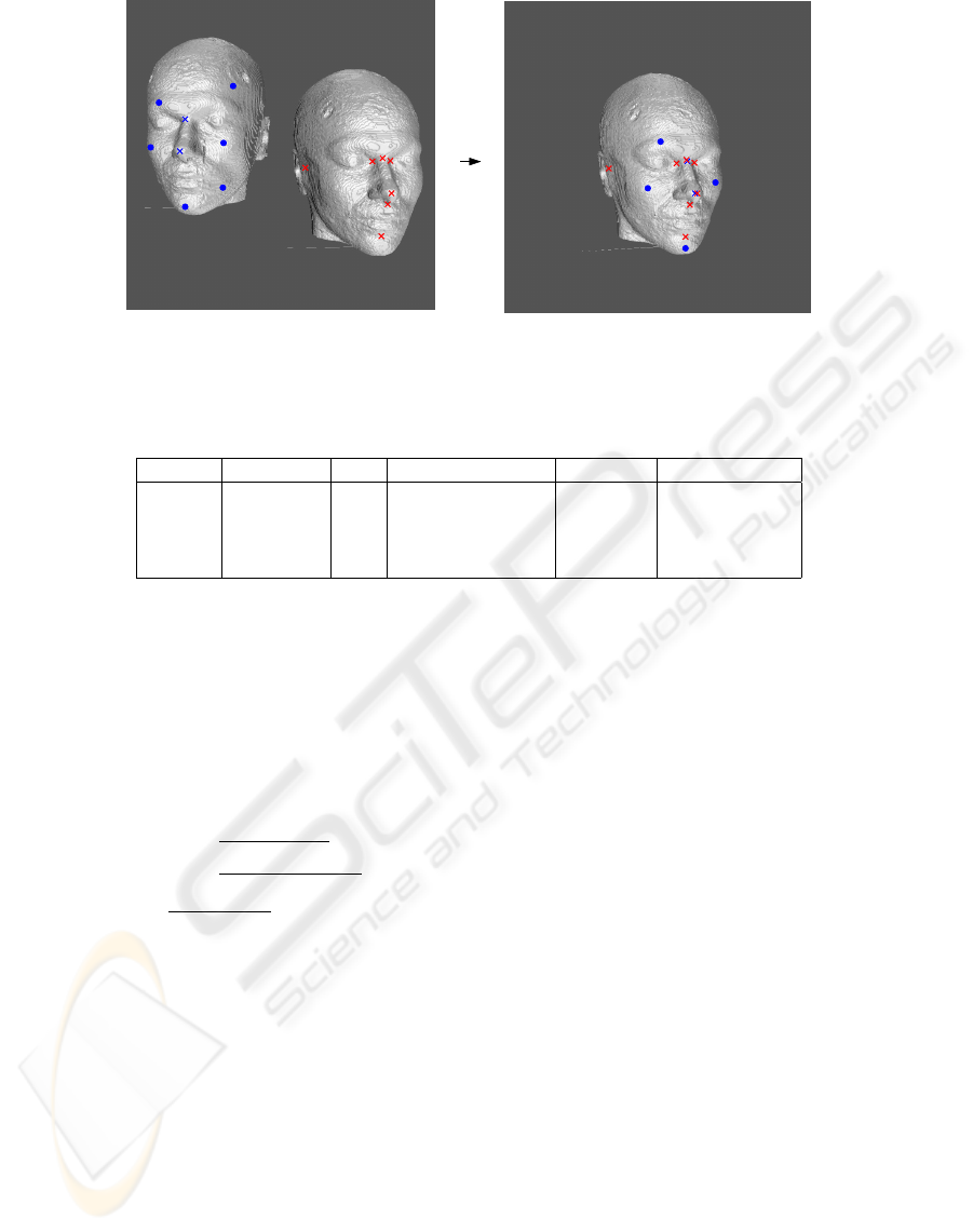
Figure 4: Registration of the head model. The characteristic points are denoted with crosses, and the non-characteristic ones
with circles.
Table 1: Some relevant parameters of the tested models. The last parameter shows the size of the subcube structure build
around the models.
model # of faces |s
c
| avg. edge length diameter # of subboxes
head 358784 10 0.988736 330.193 5120
bunny 69451 10 0.001471 0.25025 6400
cow 5804 10 0.021878 1.27111 1820
cat 671 6 0.014992 0.27041 3520
forming point set
˜
P
s
. Finally, point set
˜
P
s
was trans-
formed with a random rigid transformation T
r
, i.e.
P = {T
r
(˜p
i
) | ˜p
i
∈
˜
P
s
}.
The algorithm was tested both on noiseless and
noisy data. The tests were performed on P3,
1.27 GHz, 512 MB RAM - PC. To estimate the qual-
ity of the registration we used the following 3 mea-
sures:
• measure1 = max
i
˜p
i
−T
out
(p
i
)
diameter(S)
= max
i
˜p
i
−T
out
(T
r
(˜p
i
))
diameter(S)
,
• measure2=
−→
H (T
out
(P )S)
diameter(S)
,
• measure3 = max
i,j,i=j
(|1 − a
ii
|, |0 − a
ij
|),
a
ij
,a
ii
∈ M
out
× M
r
.
where T
out
is the output transformation given by our
algorithm, which matches the point set P with the
surface S, and M
out
and M
r
are the corresponding
matrices of the rigid transformations T
out
and T
r
re-
spectively.
The results (see tables 2, 3) show that the imple-
mentation of the semioptimal algorithm is fast, ro-
bust and gives accurate matchings. Eventual further
improvements of the accuracy can be achieved with
the λ-approximation algorithm described in the sec-
tion 3.2. Its implementation is one of the tasks for the
future. Alternatively, one can use another heuristical
approaches to improve the matching, although, as it
was previously mentioned, there is no guarantee what
kind of approximation of the optimal matching will
be achieved.
5 CONCLUSION AND FUTURE
WORK
We have given an efficient algorithms for matching a
point set and a surface, both with characteristic points.
The first nontrivial case, when the point set has two
characteristic points, was considered. We design an
algorithm which assumes that the matching positions
of both characteristic points are known. Based on
it, we show how a λ-approximation of the optimal
matching can be computed. An implementation of
this algorithm was tested on real and synthetic data,
demonstrating its efficiency, robustness and accuracy.
We would like to stress that with slight modification
of the algorithms and analysis, we can extend our re-
sults and match arbitrary point sets and shapes with
characteristic points in 3 space. The analysis shows
that the presented algorithm is competitive in com-
plexity with the solutions we have for solving the
approximate matching problem when 3 characteristic
point are known.
Further work will consist in implementation of the
grid scheme needed for the λ-approximation algo-
rithm, and designing and implementing a solution of
the matching problem when the point set contains
only one characteristic point.
REGISTRATION OF 3D - PATTERNS AND SHAPES WITH CHARACTERISTIC POINTS
399

REFERENCES
Alt, H. and Guibas, L. (1999). Discrete geometric shapes:
Matching, interpolation, and approximation. In Sack,
J.-R. and Urrutia, J., editors, Handbook of Computa-
tional Geometry, pages 121 – 153. Elsevier Science
Publishers B.V. North-Holland, Amsterdam.
Besl, P. J. and McKay, N. D. (1992). A method for registra-
tion of 3-d shapes. IEEE Trans. on Pattern Recogni-
tion and Machine Intelligence, 14(2):239–256.
Cohen-Steiner, D. and Morvan, J.-M. (2003). Restricted
delaunay triangulations and normal cycle. In Proceed-
ings of the 19th Annual ACM Symposium on Compu-
tational Geometry, pages 237–246.
Delingette, H., Hebert, M., and Ikeuchi, K. (1993). A spher-
ical representation for the recognition of curved ob-
jects. International Conference on Computer Vision,
pages 103–112.
Dimitrov, D., Knauer, C., and Kriegel, K. (2005). Match-
ing surfaces with characteristic points. In Proceed-
ings of the 21th European Workshop on Computa-
tional Geometry (EWCG), Eindhoven, Netherlands.
Hagedoorn, M. (2000). Pattern matching using similarity
measures. PhD thesis, Utrecht University.
Hoffmann, F., Kriegel, K., Sch
¨
onherr, S., and Wenk, C.
(1999). A simple and robust algorithm for landmark
registration in computer assisted neurosurgery. Tech-
nical report, Freie Universit
¨
at Berlin.
Johnson, A. and Hebert, M. (1997). Surface registration by
matching oriented points. International Conference
on Recent Advances in 3-D Digital Imaging and Mod-
eling, pages 121–128.
Kim, S.-J., Jeong, W.-K., and Kim, C.-H. (1999). Lod gen-
eration with discrete curvature error metric. In 2nd
Korea Israel Bi-National Conference on Geometrical
Modeling and Computer Graphics in the WWW Era,
pages 97–104.
Mitra, N. J., Gelfand, N., Pottmann, H., and Guibas, L.
(2004). Registration of point cloud data from a geo-
metric optimization perspective. In Symposium on
Geometry Processing, pages 23–32.
Petitjean, S. (2002). A survey of methods for recover-
ing quadrics in triangle meshes. ACM Comput. Surv.,
34(2):211–262.
Rusinkiewicz, S. and Levoy, M. (2001). Efficient variants of
the icp algorithm. In Third International Conference
on 3D Digital Imaging and Modeling, pages 145–152.
Sharir, M. and Agarwal, P. (1995). Davenport-Schinzel se-
quences and their geometric applications. Cambridge
University Press.
Sun, Y. and Abidi, M. A. (2001). Surface matching by 3d
point‘s fingerprint. In IEEE Int. Conf. On Computer
Vision, vol. II, pages 263–269.
van Laarhoven, P.-J.-M. and Aarts, E.-H.-L. (1987). Simu-
lated Annealing: Theory and Applications. D.Reidel
Publishing Company, Kluwer.
Wang, Y., Peterson, B. S., and Staib, L. H. (2000). Shape-
based 3d surface correspondence using geodesics and
local geometry. Computer Vision and Pattern Recog-
nition, 2:2644–2651.
Yamany, S. M. and Farag, A. A. (2002). Surfacing signa-
tures: An orientation independent free-form surface
representation scheme for the purpose of objects reg-
istration and matching. IEEE Transactions on Pattern
Analysis and Machine Intelligence 24(8), pages 1105–
1120.
Zhang, D. (1999). Harmonic Shape Images: A 3D Free-
form Surface Representations and Its Applications in
Surface Matching. PhD thesis, Carnegie Mellon Uni-
versity.
Zhang, D. and Hebert, M. (1999). Harmonic maps and their
applications in surface matching. In Computer Vision
and Pattern Recognition, volume 2, page 2524.
Table 2: Experimental results on noiseless data. The values
in the table are the average of the results of 100 runs of the
algorithm, each time with a newly generated point set P .
model preproc. matching # of calls of the
[s] [s] basic algorithm
head 11.433 21.556 6
bunny 2.433 4.556 7
cow 0.201 1.771 5
cat 0.04 0.951 2
measure1 measure2 measure3
head 0.000748 0.000103 0.0000037
bunny 0.004483 0.000203 0.0000663
cow 0.005954 0.001869 0.0032076
cat 0.009801 0.000899 0.0028853
Table 3: Experimental results on noisy data of the head
model. Random noise, between 0 and noise factor*average
edge length, was added to the points from P . The values
in the table are the average of the results of 100 runs of the
algorithm, each time with a newly generated point set P .
noise preproc. matching # of calls of the
factor [s] [s] basic algorithm
0 11.433 21.556 6
1 11.386 21.281 6
5 11.425 22.771 5
10 11.375 22.609 3
measure1 measure2 measure3
0 0.000748 0.000103 0.0000037
1 0.008512 0.000703 0.0000067
5 0.015954 0.001869 0.0032076
10 0.036983 0.210899 0.0048853
VISAPP 2006 - IMAGE ANALYSIS
400
