
POSE ESTIMATION USING STRUCTURED LIGHT AND
HARMONIC SHAPE CONTEXTS
Thomas B. Moeslund and Jakob Kirkegaard
Lab. of Computer Vision and Media Technology
Aalborg University, Denmark
Keywords:
Bin-picking, rotational invariant features, surface mesh, time multiplexed binary stripes, CAD model.
Abstract:
One of the remaining obstacles to a widespread introduction of industrial robots is their inability to deal with
3D objects in a bin that are not precisely positioned, i.e., the bin-picking problem. In this work we address the
general bin-picking problem where a CAD model of the object to be picked is available beforehand. Structured
light, in the form of Time Multiplexed Binary Stripes, is used together with a calibrated camera to obtain 3D
data of the objects in the bin. The 3D data is then segmented into points of interest and for each a regional
feature vector is extracted. The features are the Harmonic Shape Contexts. These are characterized by being
rotational invariant and can in general model any free-form object. The Harmonic Shape Contexts are extracted
from the 3D scene data and matched against similar features found in the CAD model. This allows for a pose
estimation of the objects in the bin. Tests show the method to be capable of pose estimating partial-occluded
objects, however, the method is also found to be sensitive to the resolution in the structured light system and
to noise in the data.
1 INTRODUCTION
One of the remaining obstacles to a widespread intro-
duction of industrial robots is their inability to deal
with 3D objects that are not precisely positioned, e.g.,
objects supplied in bins, see figure 1. The general
problem of robots handling objects located in bins or
containers is known as the bin-picking problem (Tor-
ras, 1992).
Due to multiple objects in multiple layers, occlu-
sion courses severe problems for any automatic bin-
picking system. However, two issues make the prob-
lem tractable, i) the fact that only one type of object
is usually present in a bin, and ii) the fact that a CAD
model of the object type in the bin is normally known
beforehand.
The automated bin-picking problem has been ad-
dressed using various technologies and different
methods. One approach is to first find a plane region
in an object, isolating it from the rest of the objects
using a vacuum gripper and then do the final pose
estimation using some computer vision techniques.
In (Berger et al., 2000) the plane regions are identi-
fied using a grid projector combined with a binocular
stereo setup placed above the bin. In (Saldner, 2003)
a fringe placed in front of a video projector is used
together with a high resolution camera.
A different approach is to match the CAD model
directly with the objects in the bin. This can for ex-
ample be carried out using the appearance (Balslev
and Eriksen, 2002) or circular features (Moeslund and
Kirkegaard, 2005). Alternatively, 3D data of the scene
can be found
1
and matched directly with the CAD
model, e.g., using a laser scanner (Schraft and Leder-
mann, 2003; Boughorbel et al., 2003), Active Depth
From Defocus (Ghita and Whelan, 2003), or Struc-
tured Light (Salvi et al., 2004).
1.1 Content of the Paper
In this work we address the problem of automated
bin-picking using structured light. The reason for us-
ing structured light is that it can support both the prin-
ciple of finding plane regions in objects as well as
finding the pose of an object directly in the bin. The
problem is addressed generally, in the sense that noth-
ing is assumed about the shape of the objects except
that a CAD model is present. We use one particularly
1
See (Schwarte et al., 1999; Curless, 2000) for
overviews of 3D imaging methods.
101
B. Moeslund T. and Kirkegaard J. (2006).
POSE ESTIMATION USING STRUCTURED LIGHT AND HARMONIC SHAPE CONTEXTS.
In Proceedings of the First International Conference on Computer Vision Theory and Applications, pages 101-108
DOI: 10.5220/0001367201010108
Copyright
c
SciTePress
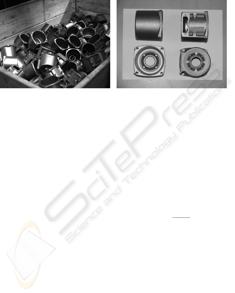
(a) A bin containing randomly organized stator housings. (b) The stator housing object shown from four different
viewpoints on a piece of A4 paper for reference.
Figure 1: Depiction of the stator housings.
object type to validate our approach. This is a sta-
tor housing object, see figure 1, produced at Grund-
fos, one of the world’s leading pump manufacturers
(www.grundfos.com, 2005).
Since the detection of plane regions has been ad-
dressed thoroughly in the past we shall in this paper
focus on finding invariant features for non-plane re-
gions. The paper is structured as follows. In section
2 it is described how the 3D surface of the objects in
the bin are reconstructed. In section 3 it is described
how the invariant features are defined and extracted.
In section 4 the matching between the CAD model
and bin data is described. In section 5 the results are
presented and finally section 6 concludes the work.
2 RECONSTRUCTING THE 3D
SURFACE
The structured light system is based on a standard
LCD projector and a single JAI monochrome CCD
camera. The encoding scheme used is Time Mul-
tiplexed Binary Stripes (Posdamer and Altschuler,
1982).
The basic principle is to project a series of pat-
terns onto the scene encoding each scene point by a
series of illumination values. The utilized patterns
are binary Gray encoded multi stripe patterns, where
the binary property refers to the use of two differ-
ent illumination values (no and full) (Valkenburg and
McIvor, 1998). More specifically the Gray codes en-
sure, that adjacent codewords only differ by a sin-
gle bit, which in turn ensures that transitions between
black and white stripes do not occur at the same po-
sition in all patterns concurrently. This principle is
illustrated in figure 2.
We use 8 bits, i.e., encoding 256 stripes with the
LSB pattern stripes being 4 pixels wide, see fig-
ure 3. Apart from the eight Gray encoded patterns
(I
0
, . . . , I
7
), two additional images are obtained of
the scene, i.e., a full-illumination (I
H
) and a zero-
illumination image (I
L
). These are used in equation
1 to compensate for ambient light and a possibly non-
constant albedo of the objects in the scene. By sub-
tracting I
L
from the pattern images, they are compen-
sated for ambient light effects. The denominator term
is proportional to the object albedo, thereby creating
an albedo normalized image, see figure 3.
J
k
=
I
k
− I
L
I
H
− I
L
(1)
2.1 Representing the Surface
After thresholding the albedo normalized images we
have a series of binary images B
0
, . . . , B
7
, which
in turn provide the projector coordinate encoding
of each pixel, see figure 3. Combining this with
a calibration between the projector and the camera
yields a number of 3D points representing the scene
(Kirkegaard, 2005). These points are subjected to a
Tessellation process, which yields a simple triangular
mesh representing the surfaces in the scene. The basic
assumption enabling the creation of the mesh is, that
world points originating from neighboring pixels in
the stripe image are also neighbors in the scene, i.e.,
these are connected.
VISAPP 2006 - IMAGE UNDERSTANDING
102
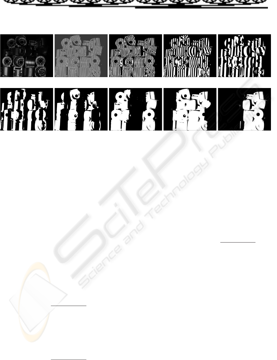
Figure 2: The principle behind the Gray coded binary representation. Each row indicates a given bit with the least significant
bits placed in the top row. Each column indicates all the bits of one codeword.
(a) I
0
(b) J
0
(c) B
0
(d) B
1
(e) B
2
(f) B
3
(g) B
4
(h) B
5
(i) B
6
(j) B
7
Figure 3: The principle of Time Multiplexed Binary Stripes when using a resolution of 8 bits.
Basically the reconstructed surface is a piecewise-
linear surface consisting of triangles. These triangles
will not be a perfect representation primarily due to
the presence of noise in the reconstruction process,
e.g., from the quantization due to the finite number of
stripes and the crude approximation of object albedo.
Therefore a smoothing of the rectangles is performed
based on the weight of the three vertices in a triangle.
The weight of each vertex, i.e., the weight of each
reconstructed 3D point, can be found from equation 1.
The value of the pixels in the J
k
images can give an
indication of the quality or fidelity of the actual pixel.
To give a quantitative measure of the pixel fidelity it is
assumed that the normalized intensity images J
k
are
contaminated by zero-mean Gaussian noise ξ(x, y)
with variance σ
2
. Given J
k
(x, y) > 0.5 the pixel
fidelity can be expressed as (Bronstein et al., 2003):
F
k
(x, y) = P {J
k
(x, y) + ξ(x, y) > 0.5} ⇔
F
k
(x, y) = Φ
0.5 − J
k
(x, y)
σ
(2)
where Φ(·) denotes the cumulative distribution
function for the normal distribution. Similar for
J
k
(x, y) < 0.5 we have:
F
k
(x, y) = P {J
k
(x, y) + ξ(x, y) < 0.5} ⇔
F
k
(x, y) = Φ
J
k
(x, y) − 0.5
σ
(3)
Errors in the most significant bit pattern effects the
stripe image more severe than errors in the less signif-
icant patterns. Therefore it is necessary to weigh the
fidelity by stripe significance. The pixel fidelity is de-
fined by (Bronstein et al., 2003) as equation 4 where
the term 2
−k
is the stripe significance weighing. The
variance σ
2
has been set to unity.
F (x, y) =
N−1
X
k=0
2
−k
F
k
(x, y) ⇔
F (x, y) =
N−1
X
k=0
2
−k
Φ
0.5 − J
k
(x, y)
σ
(4)
3 EXTRACTING FEATURES
The 3D mesh (and CAD model) provides a vast
amount of different 3D positions from where features
can be calculated. However, some locations are better
than others. For example, features on a large smooth
surface might not be the best choice since these by
nature will result in ambiguities in the matching pro-
cess. Therefore we do a segmentation of the mesh
(and CAD model) in order to find positions where the
ambiguity is low.
The general idea is to find positions where the cur-
vature of the mesh changes (Trucco and Verri, 1998)
and then calculate invariant features at these posi-
tions. The change of curvature is found by evaluat-
ing the change in the signs of the Principal Curvatures
(Kirkegaard, 2005).
POSE ESTIMATION USING STRUCTURED LIGHT AND HARMONIC SHAPE CONTEXTS
103
3.1 Shape Contexts
Before a matching between the segmented points and
the CAD model can take place a number of features
are to be extracted. We aim at a regional feature
which characterizes the surface in a small finite re-
gion around each point of interest. A regional fea-
ture is a compromise between global and local surface
features combining the noise robustness of the former
with the occlusion robustness of the latter. Concretely
we apply the Harmonic Shape Contexts as features.
Since these are a generalization of the Shape Context
features we start by explaining these.
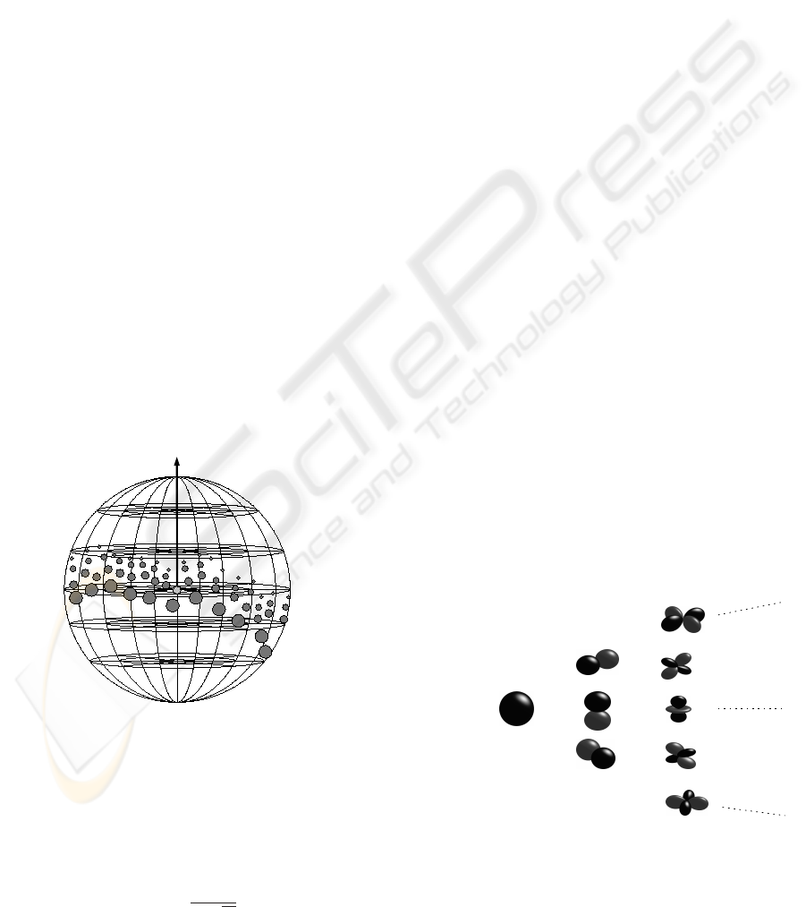
Shape contexts are regional 3D shape features
based on an oriented set of 3D points together with a
multi-dimensional histogram. The support region for
a shape context is a sphere centered at the point of in-
terest with the sphere’s north pole vector aligned with
the normal vector of the mesh in this point (Frome
et al., 2004), see figure 4.
The support region is divided linearly in the az-
imuthal (east-west) and in the colatitudinal (north-
south) directions of the sphere, while the support
sphere is divided logarithmically in the radial dimen-
sion. The number of cells are S, T , and U for the az-
imuthal, colatitudinal, and radial dimensions, respec-
tively. Altogether this division results in S × T × U
cells representing the support sphere around the point
of interest. A single cell in the sphere corresponds
to one element in a feature vector for the point of in-
terest. The support region for the shape contexts is
illustrated in figure 4.
Figure 4: The spherical support region of the shape con-
texts.
A given cell accumulates a weighted count for each
neighborhood point whose spherical coordinates fall
within the ranges of the cell. The actual contribution
(i.e., the weighting) to the cell count is given by the
function w (·) (equation 5) for a given point p
i
.
w (p
i
) =
1
ρ
i
3
√
V
(5)
The element ρ
i
in equation 5 is the local point den-
sity around the cell, while the function V denotes the
volume of the cell. The normalization by the point
density accounts for variations in sampling density,
i.e., the same surface point may have varying numbers
of neighborhood points given different image acqui-
sition viewpoints. The normalization by the volume
counteracts the effects of varying cell sizes. (Frome
et al., 2004) found empirically, that normalizing by
the cubic root of the cell volume retains discrimina-
tive power while leaving the feature robust to noise
caused by points crossing cell boundaries.
Different shape contexts cannot be compared by
simple correlation due to the shape contexts not being
rotationally invariant, i.e., there exist a degree of free-
dom in the choice of orientation of the azimuthal di-
rection. The shape contexts can however be made ro-
tationally invariant by enhancing it by use of spherical
harmonics - The Harmonic Shape Contexts (Kazhdan
et al., 2003).
3.2 Harmonic Shape Contexts
Any given spherical function, i.e., a function f (θ, φ)
defined on the surface of a sphere parameterized by
the colatitudinal and azimuthal variables θ and φ, can
be decomposed into a weighted sum of spherical har-
monics as given by equation 6.
f (θ, φ) =
∞
X
l=0
l
X
m=−l
A
m
l
Y
m
l
(θ, φ) (6)
The terms A
m
l
are the weighing coefficients of de-
gree m and order l, while the complex functions
Y
m
l
(·) are the actual spherical harmonic functions of
degree m and order l. Figure 5 depicts the principle
of expressing a given spherical function by an infinite
sum of weighted spherical harmonic basis functions.
+A
−1
1
·
+A
1
1
·
+A
2
2
·
+A
1
2
·
+A
0
2
·
+A
−1
2
·
+A
−2
2
·
+A
0
1
·f (θ, φ) = A
0
0
·
Figure 5: A spherical function expressed as a linear com-
bination of spherical harmonic basis functions. Black indi-
cates positive values and gray negative values.
VISAPP 2006 - IMAGE UNDERSTANDING
104

The following states the key advantages of the
mathematical transform based on the family of or-
thogonal basis functions in the form of spherical har-
monics. A more thorough description can be found in
(Kirkegaard, 2005).
The complex function Y
m
l
(·) is given by equation
7, where j =
√
−1.
Y
m
l
(θ, φ) = K
m
l
P
|m|
l
(cos θ) e
jmφ
(7)
The term K
m
l
is a normalization constant, while the
function P
|m|
l
(·) is the associated Legendre Polyno-
mial. The key feature to note from equation 7 is the
encoding of the azimuthal variable φ. The azimuthal
variable solely inflects the phase of the spherical har-
monic function and has no effect on the magnitude.
This effectively means that ||A
m
l
||, i.e., the norm of
the decomposition coefficients of equation 6 are in-
variant to parameterization in the variable φ.
The rotationally invariant property of the spherical
harmonic transformation makes it suitable for use in
encoding the shape context representation enabling a
more efficient comparison. For a given spherical shell
corresponding to all cells in a given radial division u,
a function f
u
is defined given by equation 8.
f
u
(θ, φ) = SC (s, t, u) (8)
where SC(s, t, u) means the shape context repre-
sentation where s (azimuthal direction), t (colatitudi-
nal direction), and u (radial division) are used to index
a particular cell.
The primary idea in the encoding process, is then
to determine the coefficients A
m
l
for each of the func-
tions f
u
for u ∈ [0; U − 1]. Based on the function in
each spherical shell, a function SH (·) can be defined
as given by equation 9.
SH (l, m, u) = ||(A
m
l
)
f
u
|| (9)
where (A
m
l
)
f
u
denotes the spherical harmonic co-
efficient of order l and degree m determined from de-
composition of the spherical function f
u
. The func-
tion SH (·) is then an invariant regional surface fea-
ture based on the principle of the shape contexts.
The actual determination of the spherical harmonic
coefficients is based on an inverse summation as given
by equation 10, where N is the number of samples
(S ×T ). The normalization constant 4π/N originates
from the fact, that equation 10 is a discretization of
a continuous double integral in spherical coordinates,
i.e., 4π/N is the surface area of each sample on the
unit sphere.
(A
m
l
)
f
u
=
4π
N
2π
X
φ=0
π
X
θ=0
f
u
(θ, φ) Y
m
l
(θ, φ) (10)
In a practical application it is not necessary (or pos-
sible, as there are infinitely many) to keep all coeffi-
cient A
m
l
. Contrary, it is assumed the functions f
u
are
band-limited why it is only necessary to keep coeffi-
cient up to some bandwidth l = B.
The band-limit assumption effectively means, that
each spherical shell is decomposed into (B + 1)
2
co-
efficients (i.e., the number of terms in the summation
P
B
l=0
P
l
m=−l
in equation 6). By using the fact, that
||A
m
l
|| = ||A
−m
l
|| and only saving coefficients for
m ≥ 0, the number of describing coefficients for each
spherical shell is reduced to (B + 1)(B + 2)/2 coef-
ficients (i.e., the number of terms in the summation
P
B
l=0
P
l
m=0
). Given the U different spherical shells,
the final dimensionality of the feature vector becomes
D = U(B + 1)(B + 2)/2 (11)
The actual comparison between two harmonic
shape contexts is done by the normalized correlation
between two D dimensional feature vectors. A corre-
lation factor close to unity resembles a good match,
while a correlation factor close to zero represent a
very poor match.
3.3 Tuning the Harmonic Shape
Contexts
The number of azimuthal and colatitudinal divisions
have no influence on the dimensionality of the har-
monic shape context feature vector. However, the
chosen divisions have influence on both the discrim-
inative power as well as the matching efficiency.
Furthermore, the number of angular divisions inflict
the required computation when determining spheri-
cal harmonic coefficients based on the shape contexts
(equation 10). As a trade-off between discriminative
power and encoding time complexity 16 colatitudinal
divisions and 32 azimuthal divisions are used. For the
radial division we empirically found that 10 divisions
spanned logarithmically between 5 and 25mm is the
best trade off. Finally the bandwidth parameter B is
set to 15 and the final number of coefficients in each
feature vector can be calculated from equation 11
10(15 + 1)(15 + 2)/2 = 1360 (12)
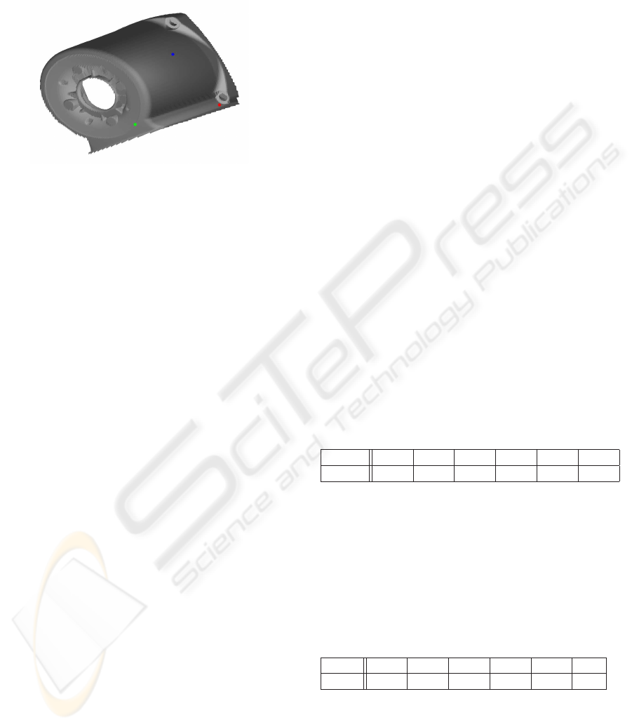
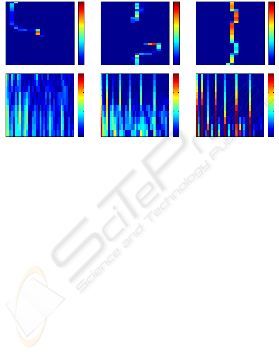
To get a better understanding of the harmonic shape
contexts we illustrate some of the coefficients in the
feature vectors for three points on a reconstructed
mesh 7. The outer shell of the shape contexts for the
three points are shown as the first row in figure 7. The
three figures depict the count for each of 32 ×16 bins
contained in the shell. The first colatitudinal bin cor-
responds to the bin around the north pole, while the
last bin corresponds to the south pole bin. The three
corresponding harmonic shape contexts for the three
POSE ESTIMATION USING STRUCTURED LIGHT AND HARMONIC SHAPE CONTEXTS
105
points are shown in the second row. The figures depict
the spherical harmonic coefficients for each of the 10
shells together with the 36 first coefficients out of the
total of 136 in each shell.
Figure 6: Object mesh with three color-marked points.
4 MATCHING
The primary purpose of extracting harmonic shape
contexts from the scene and CAD model is to perform
a matching. Due to the rotational and translational
invariance of the harmonic shape context, a feature
vector extracted from the CAD model and the scene
at positions originating from the same stator housing
object point should correlate well. Since the objects
in the scene are likely to be partial (self)occluded we
divide the CAD model into 64 sub-models seen from
different points of view and match each of these with
the extracted data.
The quality of a match cannot be judge solely by
one normalized correlation factor, i.e., it is necessary
to consider more matches at a time. This is formulated
as a graph search problem and solved using simulated
annealing (Kirkegaard, 2005).
After having found a number of matches we are left
with a number of corresponding 3D points from the
scene and CAD model. We now minimize an error
function in order to find the rigid transformation be-
tween the model and scene, i.e., the pose of the object
in the scene (Kirkegaard, 2005).
5 RESULTS
The primary evaluations performed on the method are
based on synthetic data. This is done to be able to
quantitatively judge the results of the method. We first
evaluate the method’s ability to handle occlusion, then
noise and finally the resolution of the structured light
system.
The CAD model is used to create the scene mesh
by first using a simulated structured light system (us-
ing ray-tracing) and then doing a tessellation of the
reconstructed 3D points (Kirkegaard, 2005). See fig-
ure 6 and 8 for examples.
A scene is constructed containing 12 randomly ro-
tated, translated and partial occluded stator housings,
see figure 8. The feature extraction and matching
methods are applied and the results are visually in-
spected by transforming the models into the scene us-
ing the estimated pose parameters along with compar-
ing the simulated and estimated pose parameters.
Six of the stator housings were pose estimated
correctly down to five degrees of freedom, i.e., the
”cylinder cup” where pose estimated correctly but
without the remaining cylinder axis rotation, see fig-
ure 8. Two of the stator housings were pose estimated
correctly with all six degrees of freedom. The pri-
mary reason for the many five degree of freedom re-
sults is due to the many symmetries contained in a
stator housing object, i.e., it is only the particular ter-
minal box of the stator housing object that enables the
complete six degree of freedom pose estimation.
In table 1 we list the normalized frequency of cor-
rect pose estimations as a function of the level of ran-
dom noise. The data is calculated by simulating a sta-
tor housing in 120 different configurations for each of
the different noise levels. The random noise is added
directly to the reconstructed 3D points and a correct
pose estimation is defined to be when the L2 norm
between the simulated and estimated rigid transfor-
mations is below 0.1 for both the rotation matrices
and the translation vectors.
Table 1: Normalized frequency of correct pose estimations
as a function of the level of simulated random noise [mm].
Noise 0.05 0.1 0.15 0.2 0.25 0.3
Pose 0.98 0.97 0.85 0.57 0.29 0.09
In table 2 we list the normalized frequency of cor-
rect pose estimations as a function of the resolution
in the structured light system. The latter refers to the
number of bits used to code the position of each pixel
in the stripes. The same test setup as above is used.
Table 2: Normalized frequency of correct pose estimations
as a function of the resolution in the structured light system
[bit].
Res. 10 12 14 16 18 20
Pose 0.24 0.97 0.98 0.98 0.99 1.0
6 DISCUSSION
We have in this work addressed the general bin-
picking problem where a CAD model of the object
to be picked from the bin is available beforehand.
VISAPP 2006 - IMAGE UNDERSTANDING
106
Coladitudinal bins
Azimuthal bins
2 4 6 8 10 12 14 16
5
10
15
20
25
30
0
2
4
6
8
10
12
Coladitudinal bins
Azimuthal bins
2 4 6 8 10 12 14 16
5
10
15
20
25
30
0
2
4
6
8
10
12
Coladitudinal bins
Azimuthal bins
2 4 6 8 10 12 14 16
5
10
15
20
25
30
0
2
4
6
8
10
12
Stacked Spherical Harmonic Coefficients
Radial Division
5 10 15 20 25 30 35
1
2
3
4
5
6
7
8
9
10
0
0.1
0.2
0.3
0.4
0.5
0.6
0.7
0.8
0.9
1
Stacked Spherical Harmonic Coefficients
Radial Division
5 10 15 20 25 30 35
1
2
3
4
5
6
7
8
9
10
0
0.1
0.2
0.3
0.4
0.5
0.6
0.7
0.8
0.9
1
Stacked Spherical Harmonic Coefficients
Radial Division
5 10 15 20 25 30 35
1
2
3
4
5
6
7
8
9
10
0
0.1
0.2
0.3
0.4
0.5
0.6
0.7
0.8
0.9
1
Red point Green point Blue point
Figure 7: Illustrates shape contexts (first row) and harmonic shape contexts (second row) for the red, green, and blue points on
the object mesh, respectively. Note that only the outer shell is visualized for the shape context and only the first 36 coefficients
for the harmonic shape context.
The performed tests showed that the proposed
method is capable of pose estimating 8 objects in a
scene containing 12 randomly organized and thereby
occluding stator housings for the case of simulated
noise free meshes. Even though this is only 2/3 of
the objects it is still considered a success. Firstly be-
cause only one object is required to be pose estimated
correct at a time (the scene will change after the robot
has picked one object), and secondly because they are
pose estimated very accurate even in the presence of
occlusion.
In some cases only five out of the six degrees of
freedom were correctly estimated. This is a common
problem in many bin-picking applications due to self-
symmetry but can be solve by using a two-step solu-
tion as mentioned in section 1, i.e., first isolating one
object and picking it (based on the five estimated pose
parameters) and then pose estimating it using standard
vision techniques.
When adding noise to the data table 1 showed that
the performance decreases. This is mainly due to the
fact that the harmonic shape contexts are dependent
on the direction of the normal vector. To some degree
this problem can be handled by tuning the number of
bins to the noise-level. Alternatively a better smooth-
ing mechanism is required.
From table 2 we can see that the resolution has a
high impact on the performance. Therefore a high
number of bits should be used, which again means
that the camera has to be placed closed to the objects
(allowing only a few objects to be present within the
field of view) or the resolution of the projector and the
camera has to be very high. The concrete setup in this
work only allowed a resolution of eight bits, which
turned out to be too low for the system to operate re-
liably. This result is in total agreement with table 2
where resolutions below 12 bits produce poor results.
In conclusion it can be stated that using harmonic
shape contexts is a solid approach due to the fact that
they can model any rigid object without assuming
anything about the shape of the object and can handle
partially occluded objects. This is not the case with
the traditional approaches where one assumes simple
shapes, e.g., planes or ellipses, to be present. In fact,
the harmonic shape contexts can model any free-form
object, but works best when an object contains sur-
faces with different curvatures. Therefore it seems
naturally that future general bin-picking approaches
should combine the harmonic shape contexts with ap-
proaches using more global features since these two
approaches compliment each other.
POSE ESTIMATION USING STRUCTURED LIGHT AND HARMONIC SHAPE CONTEXTS
107
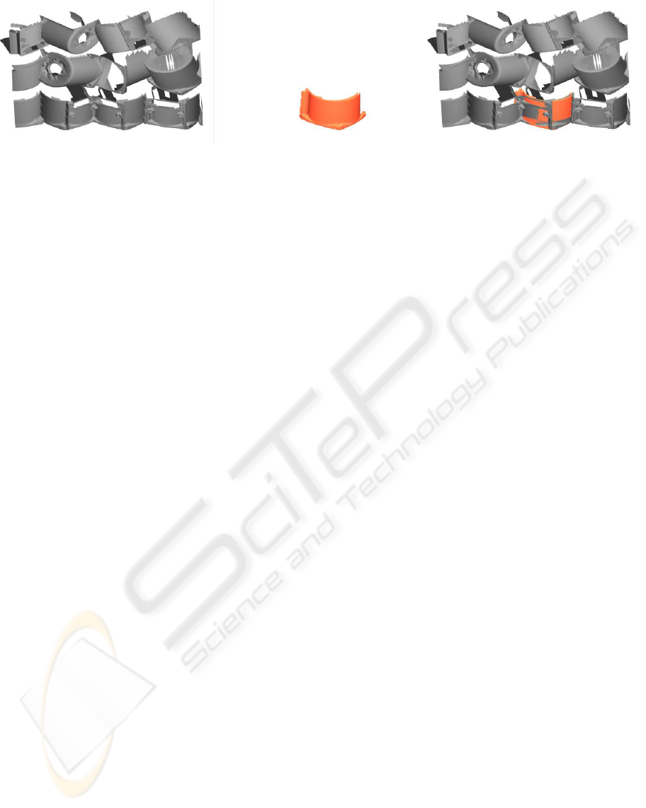
(a) The scene. (b) The (rotated and translated)
sub-model that matched best.
(c) The scene and transformed sub-model
overlaid.
Figure 8: Depiction of a correct 5 degree of freedom pose estimation.
REFERENCES
Balslev, I. and Eriksen, R. D. (2002). From belt picking to
bin picking. Proceedings of SPIE - The International
Society for Optical Engineering, 4902:616–623.
Berger, M., Bachler, G., and Scherer, S. (2000). Vi-
sion Guided Bin Picking and Mounting in a Flexi-
ble Assembly Cell. In Proceedings of the 13th In-
ternational Conference on Industrial & Engineering
Applications of Artificial Intelligence & Expert Sys-
tems, IEA/AIE2000, pages 109–118, New Orleans,
Louisiana, USA.
Boughorbel, F., Zhang, Y., Kang, S., Chidambaram, U.,
Abidi, B., Koschan, A., and Abidi, M. (2003). Laser
ranging and video imaging for bin picking. Assembly
Automation, 23(1):53–59.
Bronstein, A. M., Bronstein, M. M., Gordon, E., and Kim-
mel, R. (2003). High-resolution structured light range
scanner with automatic calibration. Technical report,
Technion - Israel Institute of Technology.
Curless, B. (2000). Overview of active vision technologies.
3D Photography - Course Notes ACM Siggraph ’00.
Frome, A., Huber, D., Kolluri, R., Bulow, T., and Malik,
J. (2004). Recognizing objects in range data using
regional point descriptors. In European Conference
on Computer Vision (ECCV), pages 224–237, Prague,
Czech Republic.
Ghita, O. and Whelan, P. F. (2003). A bin picking system
based on depth from defocus. Machine Vision and
Applications, 13(4):234–244.
Kazhdan, M., Funkhouser, T., and Rusinkiewicz, S. (2003).
Rotation invariant spherical harmonic representation
of 3d shape descriptors. In SGP ’03: Proceedings
of the 2003 Eurographics/ACM SIGGRAPH sympo-
sium on Geometry processing, pages 156–164, Sar-
dinia, Italy.
Kirkegaard, J. (2005). Pose Estimation of Randomly Orga-
nized Stator Housings using Structured Light and Har-
monic Shape Contexts. Master’s thesis, Lab. of Com-
puter Vision and Media Technology, Aalborg Univer-
sity, Denmark.
Moeslund, T. B. and Kirkegaard, J. (2005). Pose estimation
of randomly organised stator housings with circular
features. In Scandinavian Conference on Image Anal-
ysis, Joensuu, Finland.
Posdamer, J. L. and Altschuler, M. D. (1982). Surface mea-
surement by space-encoded projected beam systems.
Computer Graphics and Image Processing, 18(1):1–
17.
Saldner, H. (2003). Palletpicker-3d, the solution for pick-
ing of randomly placed parts. Assembly Automation,
23(1):29–31.
Salvi, J., Pags, J., and Battle, J. (2004). Pattern codification
strategies in structured light systems. Pattern Recog-
nition, 37(4):827–849.
Schraft, R. D. and Ledermann, T. (2003). Intelligent picking
of chaotically stored objects. Assembly Automation,
23(1):38–42.
Schwarte, R., Heinol, H., Buxbaum, B., Ringbeck, T., Xu,
Z., and Hartmann, K. (1999). Principles of Three-
Dimensional Imaging Techniques in ”Handbook of
Computer Vision and Applications”, volume 1. The
Academic Press, first edition.
Torras, C. (1992). Computer Vision - Theory and Industrial
Applications. Springer-Verlag, first edition.
Trucco, E. and Verri, A. (1998). Introductory Techniques
for 3D Computer Vision. Prentice Hall, first edition.
Valkenburg, R. J. and McIvor, A. M. (1998). Accurate 3d
measurement using a structured light system. Image
and Vision Computing, 16(2):99–110.
www.grundfos.com (2005).
VISAPP 2006 - IMAGE UNDERSTANDING
108
