RECONSTRUCTION OF ELLIPSOIDS ON ROLLERS FROM

STEREO IMAGES USING OCCLUDING CONTOURS

Sudanthi N.R. Wijewickrema and Andrew P. Papli

nski

Clayton School of Information Technology

Monash University, Victoria, 3800, Australia

Charles E. Esson

Colour Vision Systems Pty Ltd

11 Park Street, Bacchus Marsh, Victoria, 3340, Australia

Keywords:

Quadric Reconstruction, Ellipsoid Modelling, Occluding Contours, Fruit Sorting.

Abstract:

We describe the reconstruction of quadric surfaces with special attention on ellipsoids, using two different

views from calibrated cameras, given that they rest on known objects in space. The technique proposed

focuses basically on speed and efﬁciency and is suitable to be used in resource constrained environments in

real time.

We model the quadric in dual space and introduce a method of including application speciﬁc information in

the reconstruction. We also discuss a novel and fast way of adjusting the occluding contours to ﬁt the epipolar

tangency constraints before the reconstruction. We further apply this to a real-life application where ellipsoidal

fruits are modelled in 3d. Then, we analyze the error of ﬁt for the reconstructed quadrics. Although this paper

focuses on ellipsoids, it can be easily extended to incorporate the modelling of other non-degenerate quadrics

using two occluding contours in dual space.

1 INTRODUCTION

Reconstruction of quadric surfaces from occluding

contours is essential when dealing with non-textured

smooth surfaces where correspondence between fea-

tures cannot be obtained. Early works of this kind in-

clude (Giblin and Weiss, 1987) where the proﬁles of

a smooth surface was used in the reconstruction given

that the motion of the camera was small, known and

coplanar. Another approach to surface reconstruction

was later developed that could incorporate large vari-

ations of camera motion between views (Ma and Li,

1996; Mendonca et al., 2000). These were further

developed to include unknown camera motion (Cross

et al., 1999; Mendonca et al., 2000).

(Ma and Chen, 1994) introduced a non-linear re-

construction method for quadrics using perspective

views. (Ma and Li, 1996) builds on (Ma and Chen,

1994) and (Karl et al., 1994), which discusses the

reconstruction of ellipsoid surfaces from the silhou-

ettes of its orthographic projections. Both (Karl et al.,

1994) and (Ma and Li, 1996) investigate the special

case of reconstructing ellipsoids and the former shows

how this can be done with three or more orthogonal

views. The latter uses three perspective views and for

calibrated cameras, it is a linear calculation.

Techniques such as (Cross and Zisserman, 1998)

use the duality property of points and planes in the

homogeneous coordinate system. (Cross, 2000) dis-

cusses 3d surface reconstruction in detail for sin-

gle and multiple view cases and explains the use of

occluding contours in dual space and/or additional

points/planes in the calculation. (Kang et al., 2001;

Kang et al., 2003) use occluding contours to calcu-

late the tangent planes to the surface and perform the

ﬁtting of a dual quadric in the space of planes.

The aim of this paper is to discuss a method of

quadric surface reconstruction using occluding con-

tours of two perspective images focusing on the spe-

cial case of ellipsoids. Among others, we build on

the work of (Cross and Zisserman, 1998) and (Cross,

2000). The main focus of this algorithm is to maxi-

mize efﬁciency. Hence, it avoids non-linear iterative

methods and searching techniques (e.g. ﬁnding corre-

spondence). The desired application requires higher

speed, that leads to resource constraints. The solu-

tions obtained here are suitable for such an environ-

ment.

370

N. R. Wijewickrema S., P. Papli

nki A. and E. Esson C. (2006).

RECONSTRUCTION OF ELLIPSOIDS ON ROLLERS FROM STEREO IMAGES USING OCCLUDING CONTOURS.

In Proceedings of the First International Conference on Computer Vision Theory and Applications, pages 370-376

DOI: 10.5220/0001366903700376

 SciTePress

2 OVERVIEW

This section gives an overview of the method used

in the quadric reconstruction and how the paper is

structured. The algorithm uses images taken from

two non-concentric, calibrated cameras, ﬁts conics to

them and reconstructs the quadric with the use of ad-

ditional information. The technique can be summa-

rized as follows:

• Fit conics to the projections (images)

• Align the two ﬁtted conics so that they adhere to

the epipolar geometry

• Reconstruct the family of quadrics in dual space

• Select a quadric that sits on one or more known

quadric surfaces

The rest of the paper explains this method in detail.

Section 3 discusses quadrics and the duality princi-

ple and then goes on to explain how the reconstruc-

tion is done in dual space. Section 4 discusses how

to introduce application speciﬁc information into the

calculation. Section 5 addresses the implementation

speciﬁc problem of the conics not ﬁtting epipolar tan-

gency constraints. It introduces an algorithm to ad-

just them accordingly. Then, experimental results are

given in Section 6 where the algorithm is applied to

data obtained from fruit sorting applications.

3 QUADRICS AND DUAL SPACES

A quadric is a surface in 3d, represented by a 4 × 4

symmetric matrix Q. For each point X on the sur-

face, represented by a homogeneous coordinate vec-

tor X = [x y z 1]

, the following condition should

be satisﬁed.

QX = 0 (1)

The pole-polar relationship for a quadric is deﬁned as

follows. If X is a point anywhere in space, then there

exists a plane π satisfying the condition in eqn (2).

Then, X is the pole and π is the corresponding polar

plane with respect to the quadric Q. If the pole X lies

on the surface of the quadric, the polar plane π be-

comes the tangent plane to the quadric at X (Hartley

and Zisserman, 2003).

π = QX (2)

Duality in 3d is expressed as the interchangeability

of points and planes (Bruce, 1992; Hartley and Zis-

serman, 2003). Considering the equation of a plane

X = 0, we can see that interchanging the 4 ele-

ment vectors would not change the equation. So, by

using eqns (1) and (2), we get the dual quadric Q

∗

which is deﬁned by a set of planes and satisﬁes the

constraint π

∗

π = 0.

∗

= Q

−1

(3)

Alternatively, the dual can be deﬁned as the ad-

joint of the quadric Q

∗

= adj(Q) since adj(Q) =

det(Q)Q

−1

and the scale factor does not affect the

quadric equation.

A conic can be deﬁned in 2d space similar to a

quadric by a 3× 3 symmetric matrix, C. For a point in

2d x represented as a homogeneous vector of three el-

ements lying on the conic, the constraint x

Cx = 0

is satisﬁed. The pole-polar relationship is similar to

the case of a quadric where the pole is a point in 2d

and the polar is a line. l = Cx gives the relationship

between a pole and its polar line and if x is on C,

the polar line is tangent to the conic. Duality between

points and lines exists and a line conic can be deﬁned

as C

∗

= C

−1

or C

∗

= adj(C) with l

∗

l = 0

The outline of the projection of a quadric (occlud-

ing contour) is the projection of its contour generator.

The contour generator is the curve formed by the tan-

gency between the quadric and the cone of light rays

leading to the camera center. Since the contour gen-

erator arises from tangency, it is more convenient to

use the dual quadric of Q in the determination of the

projected conic. Under the camera matrix P , the pro-

jection of the quadric Q is the conic C given by eqn

(4). Here, Q

∗

and C

∗

are the duals of the quadric and

the conic respectively. Proof of this can be found in

(Hartley and Zisserman, 2003).

∗

= P Q

∗

(4)

A conic and a quadric have 5 and 9 degrees of

freedom respectively. Hence, one projection of the

quadric would impose 5 constraints on the recon-

struction. In other words, the dual of the occluding

contour conic deﬁnes 5 independent planes that the

dual quadric has to be tangent to. In the case of two

cameras though, epipolar tangency constraints dictate

that the two tangent cones generated by the two cam-

eras share two planes. Hence, in the case of two

views only 8 constraints are imposed on the quadric.

This indicates that given two views from two non-

concentric cameras, we can obtain a family of dual

quadrics as shown in eqn (5), where λ is a parame-

ter and Q

∗

and Q

∗

are known. Details of this can be

found in (Cross and Zisserman, 1998; Cross, 2000).

∗

(λ) = Q

∗

+ λQ

∗

(5)

4 TANGENCY INFORMATION

Section 3 explains the reconstruction of a family of

quadrics. To remove the ambiguity, we need to intro-

RECONSTRUCTION OF ELLIPSOIDS ON ROLLERS FROM STEREO IMAGES USING OCCLUDING CONTOURS

371

duce additional information such as another tangent

plane or points on the surface. If point information is

introduced, eqn (5) has to be inverted to get the family

of quadrics in real space giving us a cubic equation in

λ. Hence, solving the ambiguity in dual space is much

simpler and more efﬁcient.

We use the fact that most quadric surfaces in real

life would rest on some known surface, be it a plane

or another quadric in space. If the surface is a plane

(say π

), the unique quadric could be reconstructed

easily by using π

∗

= 0, giving us a value for λ

as follows:

= −

∗

(6)

But in most situations, we might just know one or

more other quadric surfaces that the quadric to be re-

constructed is tangent to. We discuss a simple cal-

culation to be used in such situations. For example,

we consider a case where the quadric lies on a set of

rollers (cylinders or cones).

In such cases, we use the fact that the quadric must

rest on some plane parallel to the xy plane between a

range of heights. The range of heights should be de-

termined from the size and orientation of the known

quadrics. For each of these heights, we calculate the

plane π

parallel to the xy plane and using eqn (6),

get a unique dual quadric. Then for each of these dual

quadrics, we check for tangency with one or more

known quadrics in space. The following section de-

scribes how this is done in a fast and efﬁcient manner.

4.1 Tangency Between Quadrics

Let the quadric to be reconstructed be Q

and the

known surface in space be Q

. For the scope of this

calculation, Q

could be any non-degenerate or de-

generate quadric while Q

should be non-degenerate.

Let X be any pole with respect to both quadrics and

π be the respective polar plane. Then, the relation-

ships in eqn (7) holds. Note that both equations give

the same plane since the scale factor µ does not affect

the equation of the plane.

π = µQ

π = Q

(7)

(µQ

− Qk)X = 0 =⇒ (µI − P )X = 0 (8)

Where,

P = Q

−1

and I is the 4 × 4 identity matrix

This is an eigensystem which has four solutions that

gives the common poles (values of X) to the two

quadrics Q

and Q

. By substituting them in eqn

(7), we get the respective polar planes.

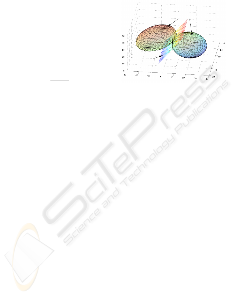
Tangent Quadrics

Coincident

Polar Planes

Coincident

Poles

Figure 1: Tangent Quadrics and coinciding Poles/Polar

Planes.

It was observed that if the quadrics are tangent to

each other, out of these four solutions, two poles (and

hence, the respective polar planes) coincide. In this

case, the coincident poles lie on the surfaces of both

and Q

fulﬁlling the tangency requirement given

in eqn (2). Figure 1 shows how two poles and polar

planes coincide in a case of tangency.

5 CONIC ADJUSTMENT

To obtain the occluding contour of the projection,

conics have to be ﬁtted to the projected images. For

this, any suitable conic ﬁtting algorithm could be

used. We use the ellipse speciﬁc algorithm discussed

in (Wijewickrema and Papli

nski, 2005) as it is more

suited for the type of application this is aimed for.

It does not require edge detection (but only a sim-

ple segmentation of the object from the background)

and uses a subset of points inside the object making it

more robust against outliers.

In real applications, the ﬁtted conics may not ad-

here to epipolar tangency constraints due to errors in

ﬁtting and the fact that the objects may not be ideal

ellipsoids. Hence, a conic correction algorithm has to

be applied on the ﬁtted conics before the reconstruc-

tion. (Cross, 2000) discusses a method of non-linear

optimization using the Levenberg-Marquardt method

for this adjustment. Alternatively, we use a more ef-

ﬁcient algorithm for conic adjustment using frontier

points as discussed in the following section.

5.1 Frontier Points

The concept of frontier points was ﬁrst introduced in

(Rieger, 1986), and was interpreted in (Porril and Pol-

lard, 1991) as the ﬁxed point on the surface of the

VISAPP 2006 - MOTION, TRACKING AND STEREO VISION

372

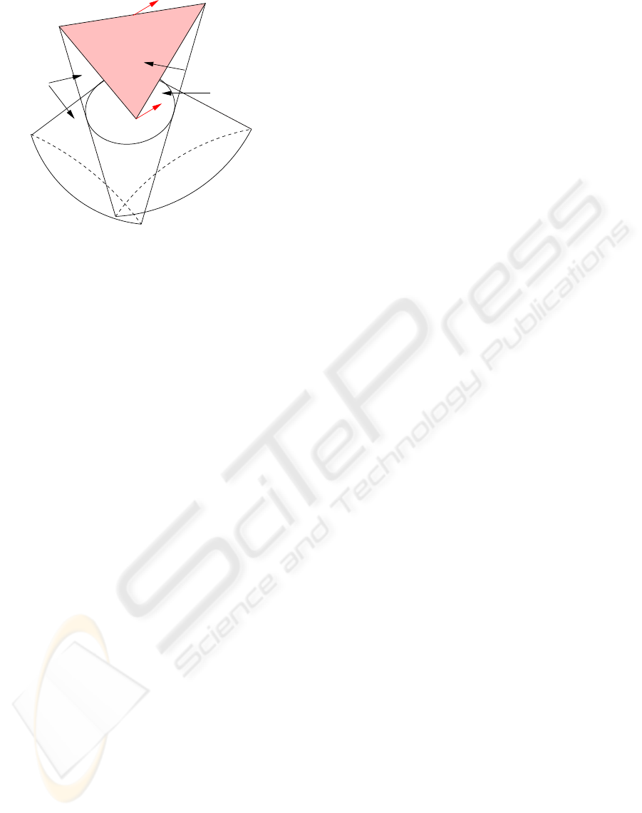
Tangent Plane at P

Cones

Quadric

Figure 2: Tangent Plane at a Frontier Point.

quadric, corresponding to the intersection of two cor-

responding contour generators. Frontier points lie on

the epipolar planes shared by the two tangent cones.

This is explained in the Occluding Edge Theorem

given in (Collins et al., 2004). It states that at the

frontier points, the tangents to the two cones and the

quadric coincide. Figure 2 shows this relationship.

We further this theorem by using the following corol-

lary.

Corollary 1: The tangent plane at a frontier point

P to the cones and the quadric, contains the vector

s joining the two cameras and the rays passing from

either camera center to P. Hence, the normal n, to

the tangent plane at P and s are orthogonal. That is:

n = 0 (9)

A cone is a degenerate quadric and hence could be

represented using a 4 × 4 symmetric matrix that sat-

isﬁes eqn (1). If it is represented by the matrix R, the

normal n to the cone at a point X would be as shown

in eqn (10), where

R is a 3 × 4 matrix consisting of

the ﬁrst three rows of R.

n = 2

RX (10)

Hence, at a frontier point X

, the normals n

and n

to the two tangent cones R

and R

would satisfy

eqn (9), giving us eqn (11).

= 0 with A =





(11)

A is a 2 × 4 matrix, the (right) null space of which

gives a one-parameter family of solutions for X

given in eqn (12). Here X

and X

are four element

vectors and γ is a scalar parameter.

= X

+ γX

(12)

Since the frontier points lie on the surface of the

cones, eqn (12) has to satisfy eqn (1) which would

yield a quadratic equation in γ. Solving for γ and

substituting in eqn (12) gives the two frontier points.

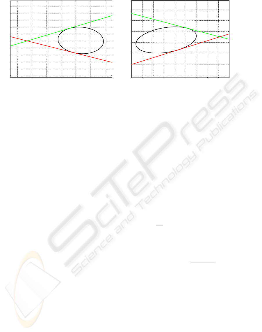
Since the plane under consideration is tangent to

the quadric, its projection on the image plane would

be tangent to the projected conic (occluding contour).

The point of contact of the conic and the tangent line

is the projection of the frontier point. The epipole

lies on this same tangent line because the tangent

plane contains the camera center of the other cam-

era as shown above. Hence, the tangents drawn from

the epipole to the conics should correspond over the

two images (same plane projected on the two image

planes). That is, they should adhere to the epipolar

geometry (Hartley and Zisserman, 2003). This is the

epipolar tangency constraint that the conics have to

satisfy. Figure 3 shows this relationship where e

and

are the epipoles and l

, l

and l

are the

corresponding epipolar tangents.

It could be seen that, if the projected conics satisfy

this constraint, the points obtained from substituting

the values of γ to either cone would yield the same

results. If not, they would essentially be different.

5.1.1 Conic Adjustment Algorithm

As mentioned above, if the projected conics do not

satisfy the epipolar tangency constraints, we get dif-

ferent sets of values for the frontier points when sub-

stituting to the equations of the two cones. For the

scope of our application, where the deviation is not

large enough to warrant iterative optimization meth-

ods, we assume that the mean of the two sets gives a

reasonable approximation.

Thus, we have two points in space that (we assume)

lie on both contour generators and hence we know

that they would be on the projected conic contours

as well. Further they would be on the common tan-

gent plane and hence the epipolar lines drawn through

these projected points should be tangent to the conic

as well. We use this property in the adjustment of the

conics.

We need to ﬁnd the conic that goes through the pro-

jected frontier points p

and p

while being tangent

to the epipolar lines l

and l

at the same points. The

tangents to the conic C can be written as shown in eqn

(13), where α

are scalars constants.

= Cp

(13)

By row scanning the conic matrix C, and using only

its unique elements, we get a vector c. Let the points

and lines be represented by p

= [p

] and

= [l

] respectively, with i = 1, 2. They

RECONSTRUCTION OF ELLIPSOIDS ON ROLLERS FROM STEREO IMAGES USING OCCLUDING CONTOURS

373

−20 −10 0 10 20 30 40

−20

−15

−10

−5

−60 −50 −40 −30 −20 −10 0 10 20 30

−30

−20

−10

Figure 3: The Epipolar Tangency Constraints.

can then be represented in matrix form, P

so that eqn

(13) could be written as α

= P

c = [c

]

0 0 0

0 p

0 0 p

0 p

Then, we can rewrite eqn (13) in the following

form, with ¯α

= −α

Nu = 0

Where,

N =



0 l



and u =

¯α

N is a 6 × 8 matrix of rank 6. Solving for the null

space of N , we get a one-parameter family of vectors.

By considering only the elements related to c, we get

the unique elements of this conic family. Here, c

and

are 6 element vectors and β is a scalar parameter.

c = c

+ βc

By rearranging the vector c to get the matrix form of

C, we get the family of conics that satisfy the epipolar

tangency constraints.

C = C

+ βC

(14)

The next step is to select the conic from this family

that suits the ﬁtted conic best. For this, from the equa-

tion of the ﬁtted conic, we generate a set of points

= [x

1] where x

is the i

point. We can

also use the set of edge points in this calculation in-

stead of points generated from the ﬁtted conic. Let

the number of points generated be n. First, we calcu-

late the algebraic distance d

= x

of each point

from the family of conics C. From eqn (14), we get:

= a

+ βb

Where,

= x

and b

= x

The error e is deﬁned as the sum of squares of alge-

braic distances for all points x

e =

i=1

+ 2β

i=1

+ β

i=1

We need to ﬁnd the value of the parameter β that min-

imizes the error e. Hence, the following has to be sat-

isﬁed.

∂e

∂β

= 2(

i=1

+ β

i=1

) = 0

This gives us the value for β that can be plugged into

eqn (14) to get the best adjusted conic.

β = −

i=1

(15)

By applying this to both projected conics, we get a

pair of conics that adhere to the epipolar tangency

constraints. They also ensure that the adjusted conics

are as close to the originally ﬁtted conics as possible.

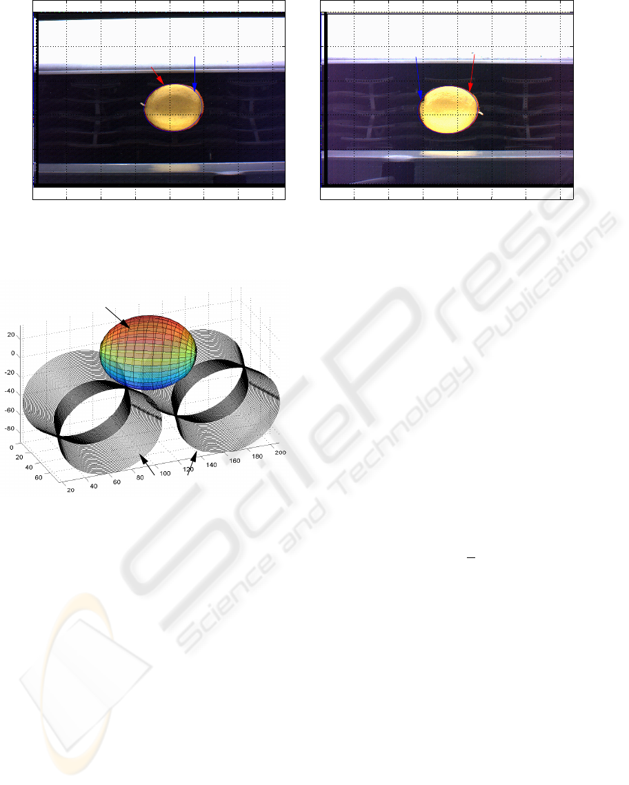
6 EXAMPLE APPLICATION

We apply our algorithm to data from a real-life appli-

cation: namely fruit sorting. Here the fruits are placed

on rollers whose dimensions and orientation in space

are known. Each fruit rests on four conic rollers and

images are captured by two cameras placed on either

side of the rollers. Images taken from the two cameras

VISAPP 2006 - MOTION, TRACKING AND STEREO VISION

374

50 100 150 200 250 300 350

100

150

200

250

Adjusted

Ellipse

Fitted

Ellipse

50 100 150 200 250 300 350

100

150

200

250

Ellipse

FittedAdjusted

Ellipse

Figure 4: Images captured by two cameras with the ﬁtted and adjusted conics.

Reconstructed

Ellipsoid

Rollers (Cones)

Figure 5: Reconstructed Ellipsoid.

along with the ﬁtted and adjusted conics are shown in

ﬁgure 4.

The roller information and the adjusted conics are

then used to reconstruct the quadric as explained in

section 3. Such a reconstructed quadric is shown in

ﬁgure 5.

6.1 Error Analysis

For the analysis of error, we use two measures: re-

projection error and volume error. The re-projection

error by itself is not a full measure of the error

involved. Any quadric selected from the family

of quadrics reconstructed using eqn (5) would be

projected on the image plane as the same conic.

Hence, the error that is calculated by comparing the

re-projection and the original ﬁtted conic (or edge

points) would just give a measure of the error involved

in conic ﬁtting and adjustment.

Hence, to get a true feel for the reconstruction

error, we need to introduce another measurement.

This is done by comparing the dimensions of the

actual ellipsoid with its reconstructed counter-part.

By calculating the volume of the actual and recon-

structed ellipsoids, we obtain this second error mea-

sure, which along with the re-projection error gives a

more rounded view of the reconstruction error.

For this experiment, we used spheres and ellipsoids

of different dimensions and placed them at different

positions and orientations. Then we calculated the re-

projection and volume errors.

The re-projection error was measured as the nor-

malized sum of squares of algebraic distances from

the ﬁtted conic to the re-projected conic. For n points

on the ﬁtted conic (or edge points), we calculate the

error as given in eqn (16).

rep

i=1

(16)

Where, d

is the algebraic distance from the i

point

to the re-projected conic.

The volume error was calculated as the percentage

error between the volumes of the actual and recon-

structed ellipsoids. The results are summarized in ta-

ble 1. The re-projection error indicates the mean of

the errors calculated for the left and right images.

7 CONCLUSION

We proposed an algorithm for reconstructing ellip-

soids given two occluding contours of views obtained

from non-concentric cameras. First we adjusted the

conics using a simple calculation as a prerequisite

to the quadric ﬁtting. Then, we discussed how the

method introduced in (Cross and Zisserman, 1998)

RECONSTRUCTION OF ELLIPSOIDS ON ROLLERS FROM STEREO IMAGES USING OCCLUDING CONTOURS

375

Table 1: Error Analysis.

Re-projection Volume

Error(10

−5

) Error(%)

Sphere 1 0.0563 3.1084

Sphere 2 2.0596 3.3040

Sphere 3 2.5063 2.6390

Ellipsoid 1 1.5880 3.4664

Ellipsoid 2 1.3303 3.1677

Ellipsoid 3 1.4047 3.2808

Ellipsoid 4 1.0186 4.8704

could be used to construct a family of quadrics in dual

space. Then we use additional application speciﬁc in-

formation so that a unique quadric can be obtained.

The basic advantage of the proposed algorithm is

that it avoids non-linear calculations. This is particu-

larly important in the type of application this is aimed

for. As shown in section 6.1, the errors involved are

quite acceptable and part of that could be contributed

to human errors involved in the obtaining of experi-

mental measurements.

The drawback in this method is that the additional

quadric surface(s), which the quadric to be recon-

structed is tangent to, must be known. This may not

be possible in some situations, making the algorithm

unsuitable. Further, the errors in the measurements

(for example, the distance of the known quadric from

the origin of the world coordinate system), account

for a large percentage of the reconstruction error. This

makes the reconstruction sensitive to human errors.

Future work related to this research is to incorpo-

rate forward movement and rotation of the quadrics

and to model the motion as well as the shape, location

and orientation. Another avenue of research would be

to come up with more accurate representations of the

surfaces and to include texture information as well.

ACKNOWLEDGEMENTS

The authors would like to thank Mr. G.C. De Silva of

Tokyo University, Japan for his invaluable input.

REFERENCES

Bruce, J. W. (1992). Lines, surfaces and duality. Mathe-

matical Proceedings of the Cambridge Philosophical

Society, 112:53–61.

Collins, S., Kozera, R., and Noakes, L. (2004). Shape re-

covery of a strictly convex solid from n-views. In

2nd International Conference on Computer Vision and

Graphics, pages 57–65, Warsaw, Poland.

Cross, G. (2000). Surface Reconstruction from Image Se-

quences: Texture and Apparent Contour Constraints.

PhD thesis, University of Oxford.

Cross, G., Fitzgibbon, A. W., and Zisserman, A. (1999).

Parallax geometry of smooth surfaces in multiple

views. In 7th International Conference on Computer

Vision, pages 323–329, Kerkyra, Greece.

Cross, G. and Zisserman, A. (1998). Quadric reconstuction

from dual-space geometry. In 6th International Con-

ference on Computer Vision, pages 25–31, Bombay,

India.

Giblin, P. and Weiss, R. (1987). Reconstruction of sur-

faces from proﬁles. In 1st International Conference

on Computer Vision, pages 136–144, London, Eng-

land.

Hartley, R. and Zisserman, A. (2003). Multiple View Geom-

etry in Computer Vision. Cambridge University Press.

Kang, K., Tarel, J.-P., and Cooper, D. (2003). A uniﬁed lin-

ear ﬁtting approach for singular and non-singular 3d

quadrics from occluding contours. In 1st International

Workshop on Higher-Level Knowledge in 3D Model-

ing and Motion Analysis, Nice, France.

Kang, K., Tarel, J.-P., Fishman, R., and Cooper, D. (2001).

A linear dual-space approach to 3d reconstruction

from occluding contours using algebraic surfaces. In

8th International Conference on Computer Vision,

pages 136–144, Vancouver, Canada.

Karl, W. C., Verghese, G. C., and Willsky, A. S. (1994).

Reconstructing ellipsoids from projections. CVGIP:

Graphical Model and Image Processing, 56(2):124–

139.

Ma, S. and Chen, X. (1994). Quadric surface reconstruc-

tion from its occluding contours. In 12th Interna-

tional Conference on Pattern Recognition, pages 27–

31, Jerusalem, Israel.

Ma, S. and Li, L. (1996). Ellipsoid reconstruction from

three perspective views. In 13th International Confer-

ence on Pattern Recognition, pages 344–348, Vienna,

Austria.

Mendonca, P. R. S., Wong, K.-Y. K., and Cipolla, R. (2000).

Camera pose estimation and reconstruction from im-

age proﬁles under circular motion. In 6th Euro-

pean Conference on Computer Vision, pages 864–877,

Dublin, Ireland.

Porril, J. and Pollard, S. (1991). Curve matching and stereo

calibration. Image and Vision Computing, 9(1):45–50.

Rieger, J. (1986). Three dimensional motion from ﬁxed

points of a deforming proﬁle curve. Optics Letters,

11(3):123–125.

Wijewickrema, S. N. R. and Papli

nski, A. P. (2005). Prin-

cipal component analysis for the approximation of an

image as an ellipse. In Proceedings of the 13th Con-

ference in Central Europe on Computer Graphics and

Visualization, pages 69–70, Plzen, Czech Republic.

VISAPP 2006 - MOTION, TRACKING AND STEREO VISION

376