SCAN-LINE QUALITY INSPECTION OF STRIP MATERIALS

USING 1-D RADIAL BASIS FUNCTION NETWORK

Afşar Saranlı

Dept. of Electrical and Electronics Eng., Middle East Technical University,

İsmet İnönü Bulv.,06531 Ankara, Turkey

Keywords: Automated Optical Inspection, Radial-Basis Functions, Gaussian Mixture Models, Image Event Detection.

Abstract: There exist a variety of manufacturing quality inspection tasks where the inspection of a continuous strip of

material using a scan-line camera is involved. Here the image is very short in one dimension but unlimited

in the other dimension. In this study, a method of image event detection for this class of applications based

on adaptive radial-basis function networks is presented. The architecture of the system and the adaptation

methodology is presented in detail together with a detailed discussion on parameter selection. Promising

detection results are illustrated for an application to grinded glass edge inspection problem.

1 INTRODUCTION

Automating the quality inspection process is an

application field of computer vision which is

increasingly becoming a major need for many

industries (Malamas et al., 2003) . This is due to

factors such as the increasing market pressure for

concurrently lowering product costs and increasing

product quality; the variation and subjectivity in the

performance of human operators in the inspection

process and the requirements on the speed-

throughput of the process. Industries where this

pressure is especially intense include, among others,

the glass manufacturing for the automotive and CRT

markets, the production of the TFT-LCD panels as

well as the inspection of textiles. (Kim et al., 2001)

(Cho et al., 2005)

Almost all of these applications require the real-

time non-contact inspection of material flowing

through the production line. A feasible way of

achieving this is through automated optical

inspection, often abbreviated as AOI, where a

camera is used to detect production defects. If the

material being inspected is moving or can be moved

at controlled speed, the use of a scan-line camera or

a TDI line-scan camera (if better illumination

sensitivity is required) is appropriate.

Systems using a scan-line camera for inspection

generates a continuous run of image data with one

comparatively smaller image axis and a

comparatively large other image axis. The digital

processing of such strips of images often require

either buffered algorithms along the scanning

direction, or preferably, scan-line based algorithms

since they are a better match for the data generation

process.

2 PROBLEM DESCRIPTION

Image processing for the inspection of a material on

the production conveyor consist of modelling the

material's normal image behaviour as it flows

through the conveyor. The task is then to perform a

detection of the anomalous or defective behaviour

on the material based on changes in the scan-line

signal.

A class of problems is when the material is a smooth

but scattering surface such as the side view of a

manufactured pipe, top view of railway tracks

(Alippi et.al., 2000) or the grinded edge of a glass

sheet. Such a scan-line camera signal is illustrated in

Figure 1.

Saranlı A. (2006).

SCAN-LINE QUALITY INSPECTION OF STRIP MATERIALS USING 1-D RADIAL BASIS FUNCTION NETWORK.

In Proceedings of the First International Conference on Computer Vision Theory and Applications, pages 19-26

DOI: 10.5220/0001366300190026

 SciTePress

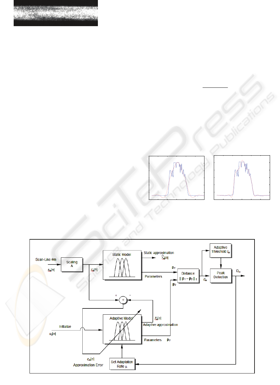
In this case, the normal signal profile has a

reasonable degree of smoothness corrupted by noise

due to the scattering properties of the surface or the

nature of the illumination. For non-defective

material, the signal behaviour does not change along

the scanning direction. Defects on the other hand be-

have as unexpected and often fast changes in the

signal behaviour along the scanning direction. When

the cross-section (or the scan-line) of the inspection

image is considered, The Radial Basis Function

network with its smoothed approximation proper-

ties appears to be ideally suited to model the

behaviour of the signal (Haykin 1999; Poggio and

Girosi 1990). In fact, RBF networks have been

successfully used in a number of detection

applications (Ahmet W. et al., 1994; Leung H. et al.,

2002; Shen M. et al., 2005).

Modelling the single scan-line with a 1-D RBF

effectively addresses the problem of suppressing the

noise while retaining the overall signal behaviour in

each scan-line. The next important problem is the

detection of the anomalous behaviour (or defects)

based on the model of the scan-line and a sequence

of the scan-line data from the image. We address

this problem in the following section by introducing

the RBF model of the scan-line a model mismatch

based detection algorithm.

3 THE RBF MODEL AND MODEL

MISMATCH DETECTION

3.1 The 1-D RBF Scan-line Model

The proposed scan-line model is given by

(1)

Based on the behaviour and the required smoothness

of the scan-line signal, a model order is chosen.

Figure 2 illustrates a model with M=7 and M=5

Gaussian basis functions superimposed with the

actual noise corrupted scan-line signal. The edge

region contains approximately 2 basis functions.

100 120 140 160 180 200 220

100

150

200

250

300

M=9 Gaus si ans along ROI ( 3 in the Edge region )

100 120 140 160 180 200 220

100

150

200

250

300

M=18 Gauss ians along ROI ( 6 in the Edge region )

Figure 2: RBF Approximations to the scan-line signal.

Figure 1: Scan-line image of material edge.

∑

⎥

⎦

⎤

⎢

⎣

⎡

−−

pnr

)(

exp][

Figure 3: The block diagram of the model mismatch based defect detection algorithm.

VISAPP 2006 - IMAGE FORMATION AND PROCESSING

3.2 Model Mismatch Based Detection

Algorithm

The defect detection algorithm is based on the

assumption that the normal edge behaviour is almost

stationary (or with very slow variation) across

subsequent scan-lines while an anomaly or defect is

an unexpected (and comparatively fast) change in

this behaviour. Therefore, we propose a detection

algorithm based on the model mismatch between a

direct static approximation to the current scan-line

data and a slowly varying (tracking) adaptive

approximation which performs a smoothing over the

history of scan-line data. A block diagram of this

model mismatch based detection algorithm is

illustrated in Figure 3.

The proposed detection algorithm maps a sequence

of scan-line image data S

[n] into a binary detection

signal D

. This is achieved by the following

procedure: Each m

1-D scan-line signal data is

modelled my a 1-D approximating RBF model

(static model) while the history of all scan-line

signal data is tracked by means of an adaptive 1-D

RBF model (adaptive model). The static model is re-

computed for each new data as the best

approximation to the data. The adaptive model is

initialized once as the best approximation to the data

and then updated for each new scan-line data by a

small amount determined by the adaptation rate

For non-defective behaviour of the signal, the static

approximation to the scan-line data is close to the

adaptive approximation to the history of the scan-

line data. Hence, the distance computed between the

two models is small.

When a defective behaviour is encountered, the

static approximation immediately reflects the defect

behaviour while the adaptive approximation,

because of its larger time constant, still reflects the

regular non-defective behaviour. Hence, a large

mismatch results between the two models, resulting

in a large model-to-model distance metric.

(a) Determination of the Static Model Parameters

The model parameters which approximate the m

scan-line data are derived by minimizing the mean-

squared-error (MSE) between the scan-line samples

and the model approximation. The total

approximation error over the m

scan-line data is

given by the expression

()

.][

][][

∑

−=

nrnrmE

(2)

To determine the parameter values minimizing the

objective function in Eq.2, we take the partial

derivatives with respect to the model parameters.

When the approximating model is also substituted in

the resulting equation, one obtains

)(

exp

)(

exp][2

][

⎟

⎠

⎞

⎜

⎝

⎛

⎥

⎦

⎤

⎢

⎣

⎡

−−

−⋅

⎟

⎠

⎞

⎜

⎝

⎛

⎥

⎦

⎤

⎢

⎣

⎡

−−

−=

∂

∑∑

pnr

(3)

which, when equated to zero gives the linear system

of equations given by

∑

∑∑

⎥

⎦

⎤

⎢

⎣

⎡

−−

⎪

⎭

⎪

⎬

⎫

⎪

⎩

⎪

⎨

⎧

⎥

⎦

⎤

⎢

⎣

⎡

−−

⎥

⎦

⎤

⎢

⎣

⎡

−−

)(

exp][

)(

exp

)(

exp

(4)

for i =1,2,...,L. This system can be expressed in

matrix form. Denoting the inside summations by α

members of an

square matrix A, the parameter

vector by p and the right hand side coefficients as

members of a vector b, this set of L equations can be

written as

bpA

⋅

. (5)

The values for the model parameters which are

optimal in the MSE sense can then be obtained as

bAp ⋅=

−1

. (6)

(b) Determination of the Adaptive Model

Parameters

The parameters of the adaptive model are once

initialized to be equal to the static model parameters

at the beginning of the algorithm processing.

However, for the remaining of the processing, they

are updated using a variation of the steepest descent

iterative optimization procedure. The procedure is

based on the popular Least-Mean Squares (LMS)

algorithm (Haykin 1996). The choice of the steepest-

descent procedure is based on the fact that we do not

require a fast adaptation but a gradual and smooth

one. The additional adaptation speed contributed by

a technique such as Recursive Least Squares (RLS)

comes at a significant computational cost and is not

justified for this application.

SCAN-LINE QUALITY INSPECTION OF STRIP MATERIALS USING 1-D RADIAL BASIS FUNCTION NETWORK

The speed of adaptation for the present procedure is

governed by an adaptation rate parameter

Specifically, for each new scan-line signal data, the

parameters of the adaptive model are updated along

the direction of the steepest descent towards the

optimum parameter values for the given data. This

direction is determined by the negative gradient of

the objective function with respect to the parameters.

Hence the update equations for the adaptive RBF

model parameters are given by

][

∇

−=

(7)

{}

111

+++

−−=

mmmmm

bpApp

(8)

where

1+m

and

1+m

are those determined from the

current scan-line data.

Standard Euclidean distance is used as the model

distance between the static and the adaptive model

and is given by

()()

()

∑

−=

−⋅−=−

alsl

asas

pppppp

(9)

(d) Detection Threshold

The model distance computed for each scan-line data

index m constitutes a model mismatch signal d[m]

which is subjected to a threshold based peak

detection to determine the binary detection D[m].

A fixed threshold can be used to perform the

detection. However an adaptive threshold scheme is

used in this study to improve the detection

sensitivity when the background noise in the

detection signal is low and to reduce false alarms

when the detection signal is noisy.

The adaptive threshold works by keeping and

updating two values, namely a partial mean level

[m] and a partial variance level

[m]. As long as

no anomaly is detected, these levels are updated

according to the equations

]1[][

]1[

⋅

mdmm

(10)

])1[]1[(][

]1[

+−++⋅

mmdmm

μσ

(11)

An anomaly is detected when the condition in Eq. 12

is satisfied. Here t

is the threshold of detection. In

this case, the adaptation of the mean and variance is

not performed for the duration of the detection so as

not to corrupt these parameters which reflect the

normal behaviour of the image.

][])[][(

mtmmd

ddd

σμ

⋅>−

(12)

(e) Post Processing of Detected Anomaly

The most important stage of the algorithm is the

detection of the anomaly in the image to indicate the

presence of a defect. However, once the defect is

located, it also needs to be sized across the strip

image and if possible, classified. This is achieved

through a second stage of post-processing, in

particular on the region indicated by the detection

stage. Although the detection algorithm proposed

can be easily applied to other application domains

with similar strip material inspection needs, this

post-processing stage is more application domain

specific. Here a solution for a particular application

domain will be considered.

As it is illustrated in the experimental results section,

we consider in particular two types of defects from

the application domain of grinded glass edge

inspection. The first type of these defects are

"shiner" defects and are composed of the lack of

proper grinding at the middle of the glass edge. This

type of defect appears dark to oblique illumination

while the properly grinded region appears light due

to the scattering of the incident illumination. The

second type of defect we consider is called an "edge

chip" and is the breaking of a small piece of glass

from the region where the glass surface and grinded

edge meet. This type of defect is usually harder to

detect since the edge signal is particularly noisy on

the sides and the chip appears as a small deviation in

the edge thickness in this region.

To determine the type and across dimension of the

defect the following procedure is applied. First, the

average values of edge starting and edge ending

values are extracted from before the beginning and

after the ending of the defect region along the

scanning direction. Then the defect region is

uniformly sampled along the scanning direction. For

each resulting scan-line segment, the signal

background level is measured and a signal threshold

is determined. The threshold is used to determine the

edge location and number and locations of threshold

crossings along the edge. For very small defect

VISAPP 2006 - IMAGE FORMATION AND PROCESSING

lengths along the scanning direction, only a single

sample from the centre may be considered for this

sampling.

Any major deviation from the average edge starting

and ending positions around the defect region is

considered as a side defect (edge chip) with its side

location information. The maximum value across the

defect-sampling of any such deviation provides the

across size of a side defect. Also, any additional

threshold crossings inside the edge identify an inside

defect (shiner). The size is measured as the

maximum separation between the beginning-

crossing and the ending-crossing across the defect-

sampling.

Parameter Selection for the Application Domain

The following is a discussion of a reasonable set of

guidelines for the selection of some algorithm

parameters:

Scaling Factor

The signal may be pre-processed with a scaling and

clipping before the detection stage is performed. For

the present application domain, from the

experimental data, it is observed that that a fixed

scaling can be used throughout the detection stage.

However, with varying camera/edge distance and

dynamic illumination power control, an adaptive

procedure may also be adopted.

Gaussian Functions

The number of the Gaussian functions used in the

approximation determine how well the edge signal is

approximated. Therefore, a larger number means a

better approximation. However, the increasing

number increases the computational complexity of

the approximation and decreases the smoothing

effect, resulting to also model the noise. This is

clearly not desirable. Therefore, the choice should be

as small as possible as long as a distance between

the static and adaptive models has a significant

enough peak in a defect region to allow detection.

M=3 or M=5 Gaussian functions whose centers are

distributed along the edge is observed to provide

good results. We have preferred an odd number of

Gaussian functions due to the symmetry of the

signal and in order to have maximum sensitivity in

the center of the image strip.

The Gaussian means are determined to provide a

uniform distribution along the edge. For the M=3

case, one mean can be placed in the center of the

edge and remaining two on the estimated edges.

Small, gradual changes on the edge will not have a

serious impact on the approximation.

The variances of the Gaussian functions are all the

same and determined by the choice of their number

and mean values. More specifically, the distance

between two adjacent Gaussian functions determines

this choice. The main criteria is to obtain a smooth

enough approximation. A variance value of

= 2.5d

where d is the distance between adjacent Gaussian

functions gives an acceptable smoothness. This

value is used for the approximations in Figure 1.

Adaptive Model Adaptation Rate

This value determines how fast the adaptive model

will follow the changes in the edge signal. Too small

a value will render the adaptive model fixed, which

will not be able to track a gradual change in the edge

signal. Too large a value will cause the adaptive

model to follow the changes in the edge signal very

closely and the model distance signal will always

remain small making detection very difficult if not

impossible. For a reasonably steady edge signal,

values in the range 0.0005 to 0.005 are found to be

reasonable choices for this application.

Detection Threshold

This threshold determines the sensitivity of detecting

a defect and also affects the size measurement of the

defect along the strip direction. As the threshold

increases, only larger disturbances on the edge will

trigger a detection. On the experimental samples

considered for this application domain, a threshold

value of 10 to 20 were appropriate choices. The

parameter range can be tuned by experimentation

with the application domain. This parameter is

considered to be the only user controllable parameter

to adjust the sensitivity of the overall system so as to

eliminate the detection of very small defects.

4 EXPERIMENTAL RESULTS

For the experiments, we consider the application

domain of grinded glass edge inspection. The edge is

illuminated with coherent light at an oblique angle.

The properly grinded edge is a scattering surface and

back scatters enough light to generate a light signal.

The grinding problems and missing parts on the

edge can be visually observed to be present in the

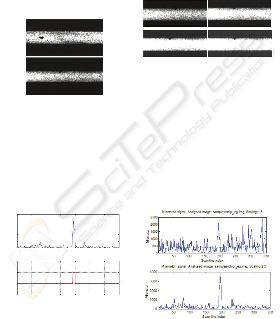
signal. Figure 4 illustrates the two aforementioned

defect types on the grinded glass edge. Figure 5

SCAN-LINE QUALITY INSPECTION OF STRIP MATERIALS USING 1-D RADIAL BASIS FUNCTION NETWORK

presents the detection stage results for the more

difficult case of an edge chip. The model mismatch

signal is illustrated in the first part of the figure

while the detection signal with the determined

beginning and ending of the image anomaly is

illustrated on the second part. From this figure, one

can observe that the model mismatch based

detection procedure successfully reduced the image

event detection into a one dimensional peak

detection task.

Figure 4: Examples of two important defect types from

grinded glass edge inspection. (a) "Shiner" grinding

problem (b) Edge chip (upper centre of the image).

Detection SNR with Signal Scaling

One interesting observation of the experimental

results is the improvement of the detection

performance of the algorithm with a software scaling

of the image signal. In reality, the noise present in

the signal is primarily due to the coherent nature of

the illumination and the resulting effects. Although

software scaling up of the image intensity may

roughly correspond to an increase in physical

illumination intensity, the noise is expected to scale

with the signal and hence no SNR improvement is

expected.

50 100 150 200 250 300 350

1000

2000

3000

4000

5000

Mismatch signal. Analysed image: samples/chip

eg.img, Scaling:2.8

Scan-line index

Mismatch

50 100 150 200 250 300 350

-1

Scan-line index

Detec tion

Figure 5: Edge chip detection. (a) the model mismatch

signal, (b) the detection signal based on a user specified

threshold.

However, it is observed that when the signal is

scaled up so that higher intensity noise is clipped at

the upper limit of the dynamic range of the signal,

this has an overall positive effect on the performance

of the model mismatch based detection. In fact, this

positive effect is also visually apparent from the

image data as can be seen in Figure 6.

Figure 6: Edge chip defect images for software scaling of

the image signal for scaling factors of s=1.0, 1.5, 2.0 and

2.5 respectively from top left to bottom right.

The model mismatch signal for the first case of

s=1.0 and the last case of s=2.5 are illustrated in

Figure 7 below. Assuming that the "signal" in the

model mismatch signal is the defect peak and the

background variation is the noise, one can conclude

that the SNR relevant to the detection algorithm

clearly improves. These results are also in agreement

with a recent study (Sakurai et al., 2002) in the field

of semiconductor inspection.

Experiments have been also conducted to assess the

sensitivity of the detection algorithm for different

defect sizes and positions on the image signal. For

this purpose, a set of simulated defects have been

generated with characteristics similar to the

observed defects. The lack of a large selection of

real defect samples have been a limiting factor at

this point. The results for these experiments are

summarized in the following sections.

Figure 7: Illustration of model mismatch signal for the

edge-chip defect for scaling factors s=1.5 and 2.5

respectively.

VISAPP 2006 - IMAGE FORMATION AND PROCESSING

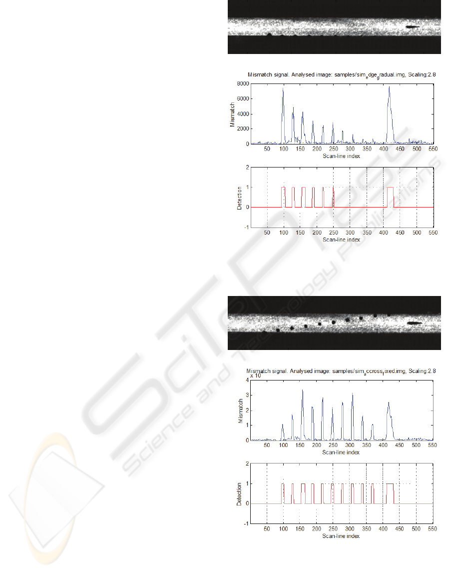
Detection Sensitivity with Defect Size

Figure 8 illustrates the set of simulated defects

generated on the grinded glass edge signal with one

real "shiner" defect sample (at the very right of the

image data). The model mismatch signal is also

illustrated in the figure and indicates the expected

degrading of the performance with defect size. A

total of 10 defects are considered on the glass edge

(which is considered to be the more challenging

case) with decreasing size from 1.3mm down to

0.1mm. The figure clearly illustrates the limit of

detection which is at defect # 6 at 0.51mm.

The experiments with the defect location across the

image data show a small amount of variation with

the sensitivity remaining at a promising level. This is

illustrated in Figure 9 for a simulated defect size of

0.91mm. Note that all defects including the ones on

both sides (corresponding to edge chip defects) are

detected for this defect size. The reason for the

sensitivity variation illustrated is the presence of a

mixture of Gaussians as the signal approximation

tool with different Gaussian mean locations across

the edge signal. The number of Gaussians have been

set to M=5 for the experiment shown in the figure. A

smaller M=3 value also leads to an operational

system with less computational complexity but with

a more severe sensitivity variation across the image.

5 CONCLUSION

A model mismatch image event detection method

based on a 1-D Radial Basis Function Network

approximator for inspecting scan-line images of strip

materials is presented. The method operates on the

principle of detecting the mismatch between a static

model derived from the scan-line and an adaptive

model which tracks the slow changes in the signal.

Thus the detector can accommodate slow variations

in the image while keeping sensitive to the fast

anomalies (defects). Experimental results on real

defect samples and simulated defects have shown

promising performance results in an application

domain of grinded glass edge inspection.

Figure 8: Experiment on detection performance with

varying defect sizes. 10 simulated edge chips and a real

"shiner" defect is present in the image.

Figure 9: Experiment on algorithm sensitivity across

the image. Simulated defect size is 0.91mm.

SCAN-LINE QUALITY INSPECTION OF STRIP MATERIALS USING 1-D RADIAL BASIS FUNCTION NETWORK

REFERENCES

Ahmed W. et al., 1994. Adaptive RBF neural network in

signal detection, Proceedings of IEEE International

Conference on Circuits and Systems, pp. 265-268.

Alippi C. et al., 2000. Composite real-time image

processing for railways track profile measurement,

IEEE Transactions on Instrumen-tation and

Measurement, Vol. 49, No. 3, pp.559-564.

Cho, C.; et al., Development of Real-Time Vision-Based

Fabric Inspection System, IEEE Transactions on

Industrial Electronics, 2005, Vol. 52, No. 4., pp.

1073-1079.

Haykin. S. 1996. Adaptive Filter Theory. (3rd edition). NJ:

Prentice Hall.

Haykin, S. 1999. Neural Networks: A Comprehensive

Foundation. Upper Saddle River, NJ: Prentice Hall.

Kim, J.H. et al., 2001 A high speed high resolution system

for the inspection of TFT LCD, Proceedings IEEE Int.

Symp. Industrial Electronics ISIE, pp. 12–16

Leung H. et al., 2002. Detection of small objects in clutter

using a GA-RBF neural network, IEEE Transactions

on Aerospace and Electronic Systems, Vol. 38, No. 1,

pp 98-118.

Malamas, E.N. et al., 2003 A survey on industrial vision

systems, applications and tools Image and Vision

Computing, 21, pp. 171-188

Poggio, T. and Girosi, F. 1990. Networks for

approximation and learning. Proceedings of the IEEE,

78(9), pp. 1481-1497.

Sakurai, K. et al. 2002. Solution of Pattern Matching

Inspection Problem for Grainy Metal Layers, IEEE

Transactions on Semiconductor Manufacturing, Vol.

15, No. 1. pp 118-126.

Shen M. et al., 2005. Real-time detection of signals in

noise using normalized RBF neural network,

Proceedings of IEEE International Workshop on VLSI

Design and Video Technology, pp. 165-168.

VISAPP 2006 - IMAGE FORMATION AND PROCESSING