
AUTOMATIC BRAIN MR IMAGE SEGMENTATION BY RELATIVE
THRESHOLDING AND MORPHOLOGICAL IMAGE ANALYSIS
Kai Li, Allen D. Malony
Department Of Computer and Information Science University of Oregon
1202 University of Oregon, Eugene, OR 97403 USA
Don M. Tucker
Electrical Geodesics, Inc.
Riverfront Research Park, 1600 Millrace Drive, Suite 307, Eugene, OR 97403 USA
Keywords:
Segmentation, brain, MR, intensity inhomogeneity, relative thresholding, mathematical morphology, skeleton-
based opening, geodesic opening, a priori knowledge, first-order logic.
Abstract:
We present an automatic method for segmentation of white matter, gray matter and cerebrospinal fluid in T1-
weighted brain MR images. We model images in terms of spatial relationships between near voxels. Brain
tissue segmentation is first performed with relative thresholding, a new segmentation mechanism which com-
pares two voxel intensities against a relative threshold. Relative thresholding considers structural, geometrical
and radiological a priori knowledge expressed in first-order logic. It makes intensity inhomogeneity transpar-
ent, avoids using any form of regularization, and enables global searching for optimal solutions. We augment
relative thresholding mainly with a series of morphological operations that exploit a priori knowledge about
the shape and geometry of brain structures. Combination of relative thresholding and morphological opera-
tions dispenses with the prior skull stripping step. Parameters involved in the segmentation are selected based
on a priori knowledge and robust to inter-data variations.
1 INTRODUCTION
Image segmentation of brain magnetic resonance
(MR) images, particularly T1-weighted MR images,
has found wide applications ranging from morphome-
tric or functional studies to neurosurgical planning.
Some brain MR image segmentation methods aim
at labeling voxels with different brain tissue types.
Typically, the tissue types of interest are white mat-
ter (WM), gray matter (GM) and cerebrospinal fluid
(CSF). Based upon the voxel classification, we can re-
construct some particular brain structures, such as the
outer and inner cortical surfaces. Some segmentation
procedures directly aim at the extraction of cortical
surfaces. These two goals roughly correspond to two
different categories of dominant segmentation meth-
ods in brain image segmentation: voxel classification
methods based on the intensity of image voxels and
deformable model-based methods considering struc-
tural information derived from the image.
Traditional voxel classification methods such as
Expectation-Maximization (EM) and fuzzy c-means
clustering are problematic in the presence of inten-
sity inhomogeneity (IIH). IIH, also referred to as bias
field, is an image artifact induced by a number of fac-
tors in image acquisition and perceived as a smooth
variation of intensity across the spatial domain of
the image. IIH correction is often performed as a
preprocessing step (Sled et al., 1998; Cohen et al.,
2000) or proceeds simultaneously with voxel classifi-
cation (Pham and Prince, 1999; Ahmed et al., 2002;
Wells et al., 1998). Brain MR image segmentation
based on deformable models (MacDonald et al., 2000;
Zeng et al., 1999; Xu et al., 1999) tracks cortical sur-
faces by exploiting information derived from the im-
age, typically edges, together with a priori knowledge
about the location, geometry, and even shape of these
surfaces. These methods usually involve minimiza-
tion of an object function that attempts to fit the model
to the image data with the regularization typically on
the surface smoothness.
Automation robustness of these segmentation
methods is not satisfactory yet mainly due to three
reasons. First, a common disadvantage of these meth-
ods is that their performance depends on the initial
segmentation state and is prone to be trapped in lo-
cal optima. Second, in those methods with regular-
ization involved, one or more parameters that control
the relative importance of regularization often have
to be empirically selected for each input image and
354
Li K., D. Malony A. and M. Tucker D. (2006).
AUTOMATIC BRAIN MR IMAGE SEGMENTATION BY RELATIVE THRESHOLDING AND MORPHOLOGICAL IMAGE ANALYSIS.
In Proceedings of the First International Conference on Computer Vision Theory and Applications, pages 354-361
DOI: 10.5220/0001366103540361
Copyright
c
SciTePress

may be sensitive to inter-data variations. This is the
case in the regularization of surface smoothness in de-
formable model-based methods and regularization of
the IIH variation smoothness in some voxel classifica-
tion methods. Third, some brain tissue segmentation
methods require a prior step of skull stripping, which
by itself is a difficult problem for complete automa-
tion (Rehm et al., 04).
W present a brain T1-weighted MR image seg-
mentation method using relative thresholding (RT)
and morphological operations that aims to improve
automation robustness in all three aspects described
above. Relative thresholding is based on image mod-
eling in terms of local spatial relationships between
near voxels and exploits structural, geometrical and
radiological a priori knowledge expressed in first-
order logic. RT makes the IIH problem transpar-
ent, avoids using any form of regularization, and en-
ables global searching for optimal solutions. Results
from relative thresholding are improved mainly us-
ing a series of morphological operations. The major
two morphological operations are what we refer to as
skeleton-based opening and geodesic opening. They
are designed to robustly remove unwanted structures
from brain structures motivated by the a priori knowl-
edge about their special shape and geometry. Parame-
ters involved in the segmentation are selected based
on a priori knowledge and robust to inter-data varia-
tions. The combination of RT and morphological op-
erations dispenses with the prior skull stripping step.
The paper is organized as follows. We first give
some basic definitions in section 2. RT and the two
morphological operations are presented in section 3
and 4 respectively. The whole segmentation pipeline
is described in section 5. The results are presented in
section 6 and the paper concludes in section 7.
2 DEFINITIONS
We first define some terms used throughout the paper.
A 3D image can be viewed as a set of cubes struc-
tured regularly, where each cube represents a volu-
metric pixel (voxel). Each voxel v has three types of
neighbors: 6 face neighbors,12edge neighbors and 6
point neighbors that share a face, an edge, or a point
with v respectively.
The 6 face neighbors are regarded as connected
to the central voxel v in 6-connectivity and form the
6-neighborhood N
6
(v) of v. The 6 face neighbors
and the 12 edge neighbors form the 18-neighborhood
N
18
(v) (18-connectivity). Finally all 26 neighbors
form the 26-neighborhood N
26
(v) (26-connectivity).
Corresponding to the three types of connectivity,
three types of distance between two voxels, D
6
, D
18
,
and D
26
, are defined as the number of steps in the
minimal path between the two voxels. Finally, we de-
fine a grid graph from an image taking each voxel as
a vertex and adding edges in terms of one of the con-
nectivies between voxels.
3 RELATIVE THRESHOLDING
Relative thresholding is characterized as differentiat-
ing the labels of near voxels by comparing their inten-
sities with respect to a relative threshold. RT exploits
various a priori knowledge in terms of a critical data
structure which we refer to as gradient graph, and is
justified by image modeling based on the spatial con-
straints on the intensities of near voxels. Optimal rel-
ative thresholds are found with a trial-and-evaluation
scheme.
3.1 A Priori Knowledge
Let g = ∇g(σ
∇
) be the gradient vector image of
g(σ
∇
). Throughout this paper, we use g(σ) to denote
the result image of performing Gaussian filtering with
standard deviation σ on the input image y. We con-
struct a directed graph G =(V,E) from g such that
each vectex v
i
∈ V corresponds to the voxel x
i
in a
region of interest R and each directed edge e
i
∈ E
emanates from v
i
to v
j
, where v
j
is the one of v
i
’s
26-neighbors that is in the direction of the gradient
vector g
i
. When v
j
is outside R, e
i
is forced to be a
loop from v
i
to itself.
The structural, geometrical and radiological a pri-
ori knowledge that we use in RT is:
• K
1
: CSF, GM, and WM are organized as a layered
structure from outside to inside;
• K
2
: The average intensities of CSF, GM, and WM
are in ascending order in T1-weighted MR images.
• K
3
: The cortex thickness is nearly uniform;
Based on the gradient graph, this a priori knowledge
is formulated as the following first-order logic: There
exist a suitable σ
∇
and p such that:
• For each GM voxel v
i
, there is a path in G of length
p from v
i
to a WM voxel;
• For each CSF voxel v
i
adjacent to GM, there is a
path in G of length ≤ p from v
i
to a GM voxel;
• There is no path from a WM voxel to a non-WM
voxel in G;
• There is no path from any non-brain voxels to WM
in G without passing CSF.
3.2 Image Modeling
We model images in terms of the spatial relationships
between voxels instead of as statistical distributions
AUTOMATIC BRAIN MR IMAGE SEGMENTATION BY RELATIVE THRESHOLDING AND MORPHOLOGICAL
IMAGE ANALYSIS
355

on the absolute voxel intensities. Our intuition is
that if the segmentation task is not beyond the hu-
man recognition capability, near voxels of the same
type should possess less difference in intensity with
respect to that of near voxels of different types. With
this type of image modeling, we attempt to avoid the
limitation imposed by the form of statistical distribu-
tions and provide a framework for introducing various
a priori knowledge into the segmentation task.
Suppose that there are K voxel types among a total
of N voxels in the space domain Ω, which represents
either the whole image or a region of interest in the
image. In brain MR image segmentation, K typically
equals to 3 and the three tissues of interest are CSF,
GM and WM. Let the coordinates of voxels be x
i
, 1 ≤
i ≤ N, and the variable and true label of each voxel
respectively be ω
i
(or ω(x
i
))∈ [1,K] and ω
i
∈ [1,K],
1 ≤ i ≤ N. Incorporating a multiplicative bias field
b
i
and an additive noise ρ, the image intensity y
i
(or
y(x
i
)), 1 ≤ i ≤ N, is modeled as:
y
i
= b
i
K
k=1
δ
k
i
y
k
i
+ ρ, where δ
k
i
=
0
ω
i
= k
1
ω
i
= k
(1)
In equation 1, δ
k
i
y
k
i
represents the component given
by tissue k in the ideal image without influence from
noise and IIH and we refer their sum
K
k=1
δ
k
i
y
k
i
as
the ideal image. Here we don’t assume any particular
statistical form on the noise term. Equation 1 is our
initial image model and will be gradually transformed
to facilitate image segmentation.
The term y
k
in equation 1 can be seen as an arbi-
trary function over the space domain governed by the
constraints on the spatial relationship between near
voxels. Generally, we think the constraints should
consider a priori knowledge about the structure and
geometry of the objects in the image as well as the
inherent image properties related to the image acqui-
sition process. In brain T1-weighted MR images, we
consider a priori knowledge K
1
and K
2
and use the
following first-order logic to describe a spatial con-
straint: any pair of near voxels from two adjacent tis-
sues differ more than any pair of near voxels in one of
the two tissues:
∀x
i
,x
j
∈ Ω ∀k ∈ [1,K] ∃T
k
∈ [0, 1)
d(x
i
,x
j
) ≤ p ⇒
(
ω
i
= k ∧ ω
j
= k +1⇒ r(y
k
i
,y
k+1
j
) <T
k
) ∧
(ω
i
= ω
j
= k ⇒ r(y
k
i
,y
k
j
) > max(T
k−1
,T
k
)) (2)
r(a, b)=
a/b a < b
b/a a ≥ b
(3)
In equation 2, T
0
and T
K
are forced to be 0, d(x
i
,x
j
)
represents the distance between voxel x
i
and x
j
, and p
is a distance threshold (a voxel cube is of unit dimen-
sion). Theoretically, any form of distance, including
Euclidean distance, can be used. However, D
6
, D
18
or D
26
distance is preferable because of the computa-
tional efficiency.
A reasonable assumption about the bias field is that
it varies slowly across the space with respect to the in-
tensity variation between different tissues in the ideal
image. We use a first-order logic to describe this as-
sumption in equation 4 without any constraints on the
variation patterns.
∀x
i
,x
j
∈ Ω ∃ ∈ (0, 1)
(1 − 1 − max(T
1
, ..., T
K−1
)) ∧
(d(x
i
,x
j
) ≤ p ⇒ r(b
i
,b
j
) >) (4)
Based on the low frequency property of the bias field,
we can safely let the function y
k
absorb the bias field
function and the bias field term can thus be dropped
from equation 1 while validity of the constraint in
equation 2 is maintained. Therefore the image arti-
fact of IIH is made transparent in our image model.
Next, we apply Gaussian filtering on the original
gray level image to counteract the noise and drop the
noise term from equation 1. Let z = g(σ
z
) be a spe-
cific blurred image. The new image model on z is:
z
i
=
K
k=1
δ
k
i
z
k
i
(5)
Here, z
k
corresponds to the contribution of tissue k to
the blurred image. After Gaussian filtering, we want
to maintain the spatial relationships between voxels,
as described equation 6.
∀x
i
,x
j
∈ Ω ∀k ∈ [1,K] ∃T
k
∈ [0, 1)
d(x
i
,x
j
) ≤ p ⇒
(
ω
i
= k ∧ ω
j
= k +1⇒ r(z
k
i
,z
k+1
j
) <T
k
) ∧
(
ω
i
= ω
j
= k ⇒ r(z
k
i
,z
k
j
) > max(T
k−1
,T
k
)) (6)
It is well-known that Gaussian filtering blurs both
homogeneous regions and edges. This leads to mainly
two types of violation to the constraint. First, for a
voxel pair (x
i
,x
j
) of different types on the opposite
sides of an edge, if they are too close to each other,
r(z
i
,z
j
) may be significantly increased such that they
may be identified as the same type. We think this ad-
verse effect can be minimized by increasing the dis-
tance between voxels pairs for comparison in the rel-
ative thresholding procedure. The second type of vi-
olation may occur when the dimension of some parts
of the structure of interest is too narrow compared to
the Gaussian filter aperture (σ
z
). We found that for
current MRI techiques, the usual resolution (around
1mm
3
) is high enough so that this violation brings
very little negative influence.
VISAPP 2006 - IMAGE ANALYSIS
356
3.3 Applying Relative Thresholds
Given two relative thresholds T
gw
between GM and
WM, and T
cg
between CSF and GM, we use two al-
gorithms for the segmentation. The inputs to both in-
clude a thresholding applying region R,acomparing
image h from which voxels are compared (we use z),
a gradient graph G constructed on R, and a relative
threshold. Based on the formulation of the a priori
knowledge, we found that it suffices for the segmen-
tation to compare only voxels pairs along paths in the
gradient graph. Each comparison involves an objec-
tive voxel and a reference voxel. In algorithm 1, the
reference voxel ref
gw
(v
i
) for the object voxel v
i
is
of distance p from v
i
along the path emanates from
v
i
. In algorithm 2, the reference voxel ref
cg
(v
i
) for
the object voxel v
i
is the farthest GM vertex along the
path emanates from v
i
. We found that it gave slightly
better results to temporarily change h(ref
cg
(v
i
)) to
h(ref
gw
(ref
cg
(v
i
)))(1−(1−T
gw
)∗2) for each com-
parison in algorithm 2. This is based on our observa-
tion that 1 minus the optimal threshold T
∗
gw
is roughly
half of 1 minus the ratio between average GM and
WM intensities.
It is easy to see that as long as our image model
(formula 6) and the a priori knowledge in 3.1 are valid
and optimal thresholds are given, the first algorithm
guarantees the exact separation between GM and WM
and the second algorithm guarantees the exact separa-
tion between CSF and GM. In practice, the segmenta-
tion accuracy depends on the goodness of the thresh-
olds and the extent to which the image model and the
a priori knowledge are valid.
Algorithm 1 GW-thresholding(R, h, G, T
gw
).
initialization: ∀x
i
∈ Rω
i
←WM;
for all x
i
∈ R do
if ω(ref
gw
(x
i
)) = GM then
ω
i
← GM;
else if r(h
i
,h(ref
gw
(x
i
))) <T
gw
then
ω
i
← GM;
end if
end for
Algorithm 2 CG-thresholding(R, h, G, T
cg
).
for all x
i
∈ R s.t. ω
i
= GM do
if r(h
i
,h(ref
cg
(x
i
)) <T
cg
then
ω
i
← CSF;
end if
end for
3.4 Finding Optimal Thresholds
The optimal thresholds are found in a trial-and-
evaluation scheme, as illustrated in algorithm 3. The-
oretically, the range for both thresholds are (0,1) and
there are infinite candidate thresholds. But in prac-
tice, we found that it suffices to try thresholds that are
multpilers of 0.01 in [0.75, 1) and [0.1, 1) for T
gw
and
T
cg
respectively. The range of T
gw
is selected based
on our observation that 1 minus the optimal thresh-
old T
∗
gw
is roughly half of 1 minus the ratio between
average GM and WM intensities, which is typically
greater than 0.5 in T1-weighted MR images.
The first input to the algorithm is the region of
interest that contain significant amount of all three
brain tissues and non-brain tissues as less as possi-
ble so that the disturbance to threshold searching is
minimized. We will refer to this region as threshold
searching region R
s
. Other inputs include a compar-
ing image h, used in the above two thresholding algo-
rithms, an evaluation image l, used for segmentation
evaluation, and a gradient graph G
s
, constructed on
R
s
. We choose to use the original intensity image y
as the evaluation image and the blurred image z as
the comparing image. After the optimal thresholds
are found, they are applied on a threshold applying
region R
a
with graph G
a
constructed on R
a
. R
s
and
R
a
are obtained with a method described in section 6.
Algorithm 3 Threshold-searching(R
s
, h, l, G
s
).
for all candidate threshold T
gw
do
apply GW-thresholding(R
s
, h, G
s
, T
gw
);
for all candidate threshold T
cg
do
apply CG-thresholding(R
s
, h, G
s
, T
cg
);
evaluate the segmentation, record the best
end for
end for
return the optimal threshold T
∗
gw
and T
∗
cg
;
Segmentation is evaluated with an objective func-
tion J as defined in equation 7:
J =
x
i
,x
j
∈R
s
ϕ
ij
|l
i
− l
j
|/
x
i
,x
j
∈R
s
ϕ
ij
, (7)
where ϕ
ij
is 1 if there is a path of length 2 in G
s
from x
i
to x
j
,or0 otherwise. Minimization of J en-
courages intensity uniformity and penalizes intensity
difference between voxels of the same type.
It is helpful to understand the mechanism of rel-
ative thresholding by comparing the result from op-
timal thresholds and those from non-optimal thresh-
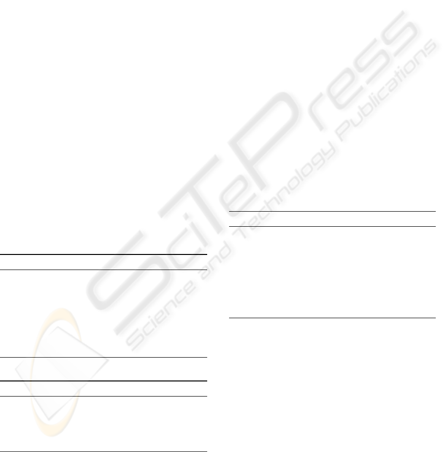
olds. Figure 1(b) shows that over-low threshold T
gw
globally makes the white matter too fat while figure
1(c) shows that over-high T
gw
globally makes it too
AUTOMATIC BRAIN MR IMAGE SEGMENTATION BY RELATIVE THRESHOLDING AND MORPHOLOGICAL
IMAGE ANALYSIS
357
thin. In either case, the GM/WM boundary drifts
away the correct situation in different directions.
(a) Input image (b) T
gw
=0.68, T
cg
=0.7
(c) T
gw
=0.93, T
cg
=0.7 (d) T
gw
=0.86, T
cg
=0.7
Figure 1: Analysis of relative thresholding applied on a
phantom image with optimal T
∗
gw
=0.86 and T
∗
cg
=0.7.
Due to various violation to our image model and a
priori knowledge, segmentation errors arise even with
optimal relative thresholds. A major error involves
labeling non-brain voxels as brain voxels which are
connected to the true brain voxels. This type of er-
ror will be corrected by morphological operations de-
scribed in the next section. Another typical error is
missing certain fine WM structures which are recov-
ered with some ridge detection operations. Examples
of such errors are circled in figure 3(b). The whole
segmentation pipeline will be presented in section 5
4 MORPHOLOGICAL IMAGE
ANALYSIS
In this section, we present the skeleton-based open-
ing operation for eliminating false WM voxels and
the geodesic opening operation for eliminating false
GM and CSF voxels. Both operations are motivated
by the a priori knowledge about the shape and geom-
etry of brain structures. Before describing these two
operations, we need to first have a review of geodesic
dilation and geodesic erosion.
Geodesic dilation(erosion) (Soille, 2003) involves
two input images: a marker image and a mask image.
The geodesic dilation(erosion) of size 1 of the marker
image f with respect to the mask image m is defined
as the intersection(union) between m and the elemen-
tary dilation(erosion) of f. A usual constraint here is
that the mask image m is the superset(subset) of the
marker image f in geodesic dilation(erosion). The
geodesic dilation(erosion) of size n of a marker im-
age f with respect to a mask image m is obtained by
performing n successive geodesic dilations(erosions)
of size 1 of f with respect to m.
4.1 Skeleton-based Opening
Skeleton-based opening considers the characteristics
of the special surface-like shape of the WM and the
strong connectivity of the WM structure. It provides
a large parameter range that gives rise to acceptable
results. The main idea is that a special erosion and
geodesic dilation are performed on the surface skele-
ton of the object instead of on the object itself. The
algorithm consists of the following 5 steps.
1). Compute the reversible surface skeleton S of a
3D object by iterative thinning of the distance trans-
forms with the method described in (Svensson, 2001).
The skeleton is at most of two-unit thickness and is
further thinned to two unit-thickness skeletons S
1
and
S
2
, where S
1
∪S
2
= S, with the sub-iteration method
described in (Borgefors et al., 1999).
2). Iteratively erode S
1
and S
2
based on the
classification of the skeleton points. We use the
method presented in (Saha and Chaudhuri, 1996)
classifying the skeleton points into the following
types: I(Isolated), SE(edge point of surfaces), S(inner
point of surface), SS(junction point of surfaces),
SC(junction point of surfaces and arcs), CE(arc end
point), C(inner point of arcs), CC(junction point of
arcs). In each iteration, a skeleton point is eroded only
if its type is I, SE, CC, CE, C, or CC. The number of
iterations n is taken as the parameter of the opening
operation.
3). Find the largest components, C
1
and C
2
, of the
eroded skeletons respectively.
4). Compute the geodesic dilation of size n of C
1
and C
2
with respect to S
1
and S
2
respectively. The
dilated skeletons are D
1
and D
2
respectively.
5). Recover the binary object from D
1
∪ D
2
by re-
verse distance transforms. Any voxels in the original
object but not in the new object are discarded.
Our experiments of applying SBO on a set of WM
groundtruths with resolution around 1mm
3
demon-
strated the following common behaviors of SBO:
there are two parameter threshold d
1
(around 13) and
d
2
(around 27) such that: 1) when n<d
2
, all fore-
brain WM voxels remain almost intact in the result
of SBO; 2) when n>d
1
the brainstem and cerebel-
lum (BC) get dropped. Therefore, we can see that
SBO provides two large parameter ranges for elimi-
nating false WM voxels ([1,d
1
)) and BC WM voxels
VISAPP 2006 - IMAGE ANALYSIS
358

([d
1
,d
2
)) as long as the connectivity of the WM struc-
ture maintains well in the prior segmentation results.
4.2 Geodesic Opening
Geodesic opening also involves a marker image f and
a mask image m ⊂ f. An example is that m denotes
the WM voxel set and f denote the union of GM voxel
set and m. Another example is that m denotes the
union of GM and WM while f denotes the union of
CSF, GM and WM. A geodesic opening of size n con-
sists of three steps: a geodesic erosion of size n of f
with respect to m resulting in image f
e
, identifying
the largest connected component f
c
of f
e
and elim-
inating any other components in f
e
, and a geodesic
dilation of size n of f
c
with respect to f.
Geodesic opening has the effect of smoothing the
geodesic distances of points in f − m from m by
eliminating protrusion voxels from f. Here, geodesic
distance of a point v in f − m from m is the min-
imum length of paths from v to m via only points
in f . This smoothing effect is particularly helpful
for elimination of unwanted structures from the ini-
tial GM and CSF voxel sets given by relative thresh-
olding due to the following characteristics about GM
and CSF structures: the thickness of human cortex is
nearly uniform and CSF fills concave spaces forming
a smooth boundary of the whole brain volume.
5 BRAIN MRI SEGMENTATION
In this section, we present the integration of RT
and morphological operations into a whole brain
MRI segmentation pipeline, as shown in figure 5.
The pipeline starts with binarization of the input
image and computing the threshold searching re-
gion (R
s
) and the threshold applying region (R
a
)
from the foreground. We simply apply traditional
thresholding with a threshold T
b
for the binariza-
tion. The background intensities are modeled as a
constant field a plus a noise term in Rayleigh sta-
tistics. The background pdf is thus f (x|a, b)=
((x − a)/b
2
)e
−(x−a)
2
/2b
2
. The parameters of the
pdf are estimated based on what we refer to as au-
tomatic training, which consists of following three
steps. First, N
b
voxels of lowest intensity in g(σ
b
)
are selected as the training set. Second, the original
intensities of the voxels in the training set are used
as the sample data to estimate the parameter a
∗
and
b
∗
that give rise to the maximum likelihood. Third, a
threshold T
b
= a
∗
+3b
∗
is applied on y = g(0), g(δ),
g(2δ), ..., g(σ
b
= nδ) for the binarization resulting
in a new training set of background voxels. Here, a
voxel is taken as background if its intensity in any of
g(kδ)|
0≤k≤n
is less than T
b
. The second and third
step can be repeated multiple times to get improved
results.
Ridge
detection
Relative
thresholding
Graph cut
operation
Morphology
thresholding
training−base
d
Automatic
R
CSF segmentation
GM segmentation
Binarization
WM segmentation
Relative thresholding
andCompute R
a
S
Figure 2: Segmentation pipeline.
We obtain a head mask image and take it as the
threshold applying region R
a
by applying SBO and
morphology closing on the foreground. R
s
is ob-
tained by taking the intersection between the result of
applying morphology erosion on R
a
and those vox-
els within a distance d
1
s
from the superior end of the
head. The erosion kernel ball radius d
2
s
is selected
based on the a priori knowledge on skull thickness.
A threshold searching region is shown in figure 3(a).
A threshold applying region is shown in figure 3(b) as
all colorful areas.
After T
∗
gw
and T
∗
cg
are found on R
s
, apply them on
R
a
with the comparing image being z = g(σ
z
). Let
S
z
w
, S
z
g
, S
z
c
, denotes the result voxel set of WM, GM,
and CSF respectively. We also use them to denote the
corresponding mask images. An example of the result
in shown in figure 3(b). Note that some missing fine
WM structure are marked with cyan circles. Next,
we use two ridge detection operations to recover these
missing fine WM structures.
For each voxel x
i
∈ S
z
g
, the first ridge detection
operation checks the 26-neighborhood of x
i
. Among
all neighbor pairs of opposite direction from x
i
, the
pair (x
j
,x
k
) with maximum value of |z
i
− z
j
| + |z
i
−
z
k
| is selected. If z
i
>z
j
and z
i
>z
k
, then x
i
is
taken as a WM ridge point, removed from S
z
g
, and
put into S
r
.Ifz
i
<z
j
and z
i
<z
j
, then x
i
is taken
as a valley point and put into S
v
. Figure 3(c) shows
the augmentation of WM ridge points.
The second operation depends on a masked
Gaussian filtering. We use
g(σ, m) to denote the re-
sult image of applying masked Gaussian filtering on
the input image y with standard deviation σ and mask
image m. Only voxels in the mask are filtered and
any voxels outside the mask are not counted in the
convolution calculation. A masked Laplacian filter-
ing is then performed on
z = g(σ
z
,S
z
w
∪ S
z
g
− S
v
)
with mask S
z
g
−S
v
to recover more missing WM vox-
els. The Laplacian of each voxel x
i
∈ S
z
g
− S
v
is
x
j
∈N
6
(x
i
)∧x
j
∈S
z
w
∪S
z
g
−S
v
(z
j
− z
i
). If the laplacian
AUTOMATIC BRAIN MR IMAGE SEGMENTATION BY RELATIVE THRESHOLDING AND MORPHOLOGICAL
IMAGE ANALYSIS
359
value is less than 0, x
i
is taken as a WM ridge point,
removed from S
z
g
, and put into S
lr
. The Laplacian
ridge points are mainly used to enhance the connec-
tivity of the WM structure and may incorporate many
false WM voxels. They will be eliminated as the final
step of WM segmentation.
We apply SBO on S
z
w
∪ S
r
∪ S
lr
with parameter
d
1
w
resulting in a WM set S
1
w
with non-brain vox-
els removed. The same operation is performed with
a greater parameter d
2
w
resulting in S
2
w
with further
removement of brainstem and cerebellum(BC). Then
we get the forebrain WM set as S
f
w
by subtracting the
largest component in S
1
w
− S
2
w
from S
1
w
and the BC
WM set as S
bc
w
= S
1
w
− S
f
w
. Result of applying SBOs
is illustrated in figure 3(d).
The separation between forebrain WM and BC
WM is calibrated by a graph-cut based method. First
we construct a grid graph in 26-connectivity from
S
1
w
. Then all vertices in S
bc
w
are contracted into a
source terminal and all vertices in S
f
w
that are of geo-
desic distance greater than a threshold d
f
from S
bc
w
are contracted into a sink terminal. Finally we com-
pute the minimum graph cut between the source and
sink terminal. It is demonstrated in (Boykov and Kol-
mogorov, 2003) that as long as the edge weights in
the grid graph are set to be inversely proportional to
their length, the graph cut can approximate the area of
the cut surface. In this way, the initial forebrain/BC
separation is substituted with a smaller and more reg-
ular cut surface and S
f
w
and S
bc
w
are updated accord-
ingly. Finally, we remove Laplacian ridge points by
subtracting S
lr
from S
f
w
. All discarded WM voxels
from S
z
w
that have a path in G
a
to S
f
w
or S
bc
w
are de-
graded to S
z
g
. Final result of WM segmentation is
shown in figure 3(e).
Given the result of WM, GM segmentation is made
easier considering the a priori knowledge on the
nearly uniform cortex thickness. First, we obtain an
initial forebrain GM set S
f
ig
⊂ S
z
g
by extracting all
voxels in S
z
g
that have a path to S
f
w
in G
a
of length
less than d
1
g
. In a similar way, we can get the BC GM
voxel set S
bc
g
and the total BC set S
bc
= S
bc
g
∪ S
bc
w
.
False GM voxels in S
f
g
are removed by a series of
geodesic openings with size being 1, 2, ..., d
1
g
. Let the
result be S
f
g
. These operations may over-smooth the
geodesic distances of GM voxels to the WM set. We
improve the result by simply computing the geodesic
dilation of size d
2
g
d
1
g
of S
f
g
with respect to S
f
ig
.
Any discarded WM voxels from S
f
ig
that have a path
in G
a
to S
f
w
are degraded to CSF and put into S
z
c
.
To improve the CSF voxel set given by relative
thresholding, we first extract the subset S
c
⊂ S
z
c
in
which each voxels has a path in G
a
to S
f
g
∪ S
f
w
∪ S
bc
.
From S
c
we build a normal distribution for CSF voxel
intensities using a similar automatic training method
to that used for image binarization (see the first para-
graph of this section). The distribution then guides
incorporation of additional CSF voxels. The up-
dated CSF voxel set S
c
is finally processed by a se-
ries of geodesic openings smoothing the brain volume
boundary. A example of final result is shown in fig-
ure 3(f) and two real image segmentation results are
shown in figure 4.
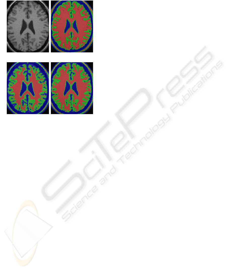
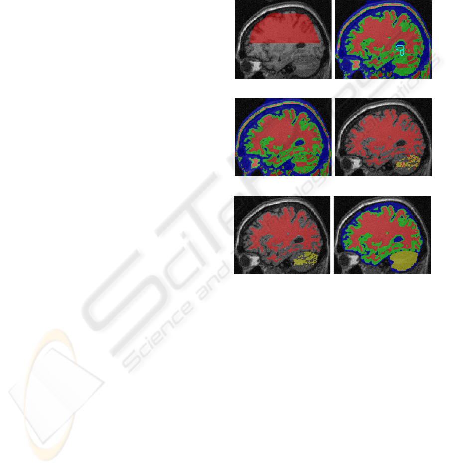
(a) Input image and R
s
(b) RT result on R
a
(c) First ridge detection (d) Applying SBO on WM
(e) Graph cut result (f) Final result
Figure 3: Segmentation of a phantom brain (IIH level =
40%, noise level = 9%). WM, GM, CSF, and BC are col-
ored with red, green, blue, and yellow respectively.
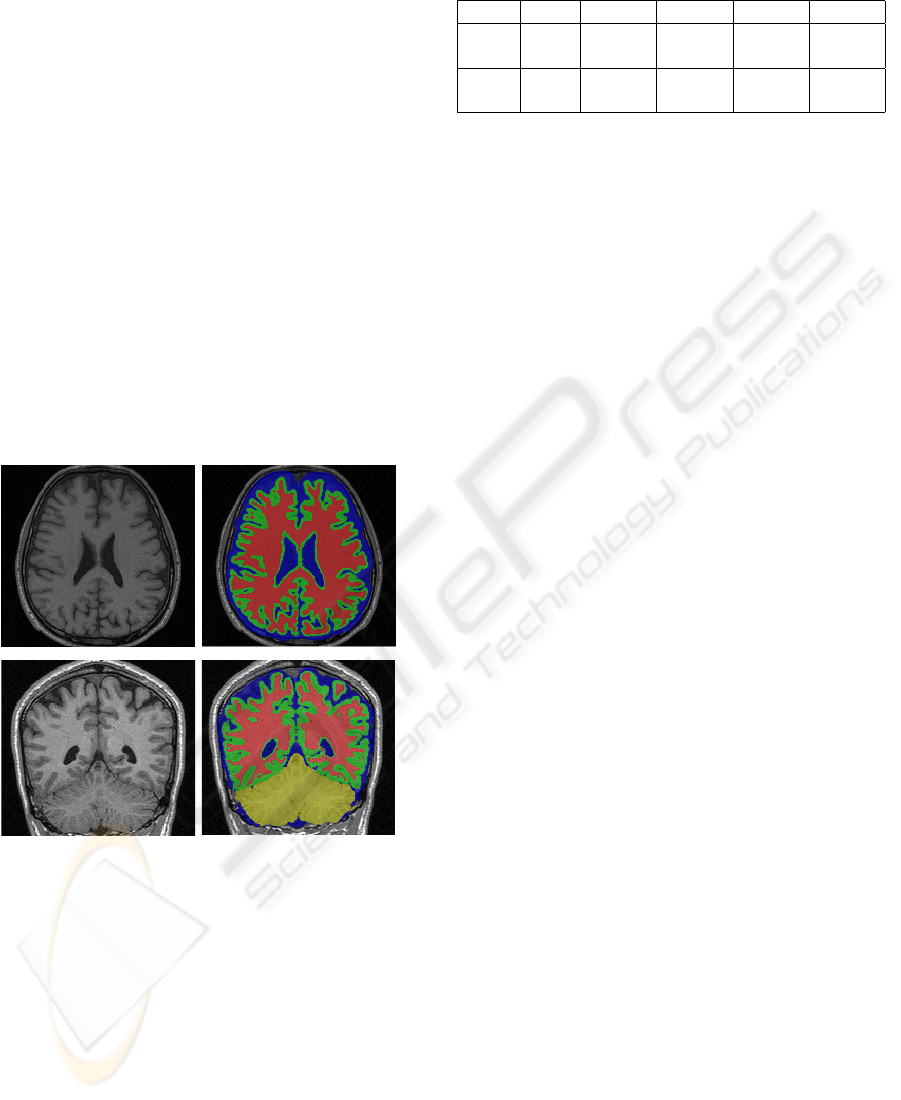
6 RESULTS
We have tested the segmentation algorithm against
a set of phantom brains as well as 6 real images
from 4 subjects scanned at 3 different MR machines.
Some examples of the results are shown in figure 4.
The resolution of the images are between 1.3mm
3
and 1mm
3
. The average running time is less than
8 minutes on a single 1.3GHz Power4 processor.
Searching for the optimal relative thresholds takes
about 1.5 minutes. We use exactly the same set of
parameters for all these images. Some important pa-
rameters are selected as follows: σ
z
=1, σ
∇
=2,
p =8, d
1
s
=95, d
2
s
=25, d
1
w
=4, d
2
w
=18, d
1
g
=15,
and d
2
g
=2. We think this set of parameters work
VISAPP 2006 - IMAGE ANALYSIS
360
for all input images with resolutions around 1mm
3
,
which is typical for current MR techniques. The only
place where user intervention may be needed is deter-
mining the transaxial dimension and the superior side
to obtain the threshold searching region. This infor-
mation can also be obtained by computation or from
the input file.
To evaluate segmentation, we use a metric over-
lap, same as the Tanimoto coefficient (Duda and
Hart, 1973), comparing two segmentations for a given
voxel type labeling as the sum of voxels that both
have the same label in each segmentation divided by
the sum of voxels where either segmentation has the
label. Table 1 list the overlaps of WM and GM re-
spectively between the groundtruth and our results
on phantom brains corrupted with partial volume ef-
fect, various levels of IIH and noise (Cocosco et al.,
1997). The noise level represents the percent ratio
of the standard deviation of the white Gaussian noise
versus the signal for a reference tissue. For a IIH level
x, the multiplicative IIH field has a range of values of
1 − x...1+x over the brain area.
Figure 4: Results of two real images.
7 CONCLUSION
We have demonstrated a new automatic brain MRI
segmentation method with relative thresholding and
morphological operations. Relative thresholding
makes IIH transparent and allows global searching
for optimal solutions. Prior skull stripping is not re-
quired. Parameters are selected based on a priori
knowledge and are robust to inter-data variations.
Table 1: WM and GM overlaps on a set of phantom brains.
Type IIH N=3% N=5% N=7% N=9%
WM 20% .8931 .8899 .8897 .8812
WM 40% .8926 .8899 .8832 .8824
GM 20% .8100 .8043 .8060 .7967
GM 40% .8074 .8060 .8048 .7996
REFERENCES
Ahmed, M. N. et al. (2002). A modified fuzzy c-means
algorithms for bias field estimation and segmentation
of mri data. IEEE Trans. Medical Imaging, 21(3).
Borgefors, G. et al. (1999). Computing skeletons in threee
dimension. Pattern recognition, 32(7).
Boykov, Y. and Kolmogorov, V. (2003). Computing geo-
desics and minimal surfaces via graph cuts. In Inter-
national Conference on Computer Vision.
Cocosco, C. A. et al. (1997). Brainweb: Online interface to
a 3d mri simulated brain database. NeuroImage, 5(4).
Cohen, M. S. et al. (2000). Rapid and effective correction
of rf inhomogeneity for high field magnetic resonance
imaging. Human Brain Mapping, 10.
Duda, R. and Hart, P. (1973). Pattern Classification and
Scene Analysis. Wiley, New York.
MacDonald, D. et al. (2000). Automated 3-d extraction of
inner and outer surfaces of cerebral cortex from mri.
NeuroImage, 12(3).
Pham, D. L. and Prince, J. L. (1999). An adaptive fuzzy c-
means algorithm for image segmentation in the pres-
ence of intensity inhomogeneities. Patt. Rec. Let.
Rehm, K. et al. (04). Putting our heads together: a consen-
sus approach to brain/non-brain segmentation in t1-
weighted mr volumes. NeuroImage, 22.
Saha, P. K. and Chaudhuri, B. B. (1996). 3d digital topology
under binary transformation with applications. Com-
puter vision and image understanding, 63(3).
Sled, J. G. et al. (1998). A nonparametric methods for au-
tomatic correction of intensity nonuniformity in mri
data. IEEE Trans. Medical Imaging, 17.
Soille, P. (2003). Morphological image analysis. Springer-
Verlag.
Svensson, S. (2001). Reversible surface skeletons of 3d ob-
jects by iterative thinning of distance transforms. In
G.Bertrand et al. (Eds.): Digital and Image geometry,
LNCS 2243.
Wells, W. M. et al. (1998). Adaptive segmentation of mri
data. IEEE Trans. Medical Imaging, 15.
Xu, C. Y. et al. (1999). Reconstruction of the human cere-
bral cortex from magnetic resonance images. IEEE
Trans. Medical Imaging, 18.
Zeng, X. et al. (1999). Segmentation and measurement of
the cortex from 3-d mr images using coupled-surfaces
propagation. IEEE Trans. Medical Imaging, 18(10).
AUTOMATIC BRAIN MR IMAGE SEGMENTATION BY RELATIVE THRESHOLDING AND MORPHOLOGICAL
IMAGE ANALYSIS
361
