
EFLAM: A MODEL TO LEVEL-LINE JUNCTION EXTRACTION
N. Suvonvorn
Institut d’Electronique Fondamentale, Universit
´
e Paris 11
B
ˆ
atiment 220 - 91405 Orsay Cedex
B. Y. Zavidovique
Institut d’Electronique Fondamentale, Universit
´
e Paris 11
B
ˆ
atiment 220 - 91405 Orsay Cedex
Keywords:
Level-line, level sets, corner, point of interest, extraction.
Abstract:
This paper describes an efficient approach for the detection of level-line junctions in images. Potential junc-
tions are exhibited independent from noise by their consistent local level-variation. Then, level-lines are
tracked through junctions in descending the level-line flow. Flow junctions are extracted as image primitives
to support matching in many applications. The primitive is robust against contrast changes and noise. It is
easily made rotation invariant. As far as the image content allows, the spread of junctions can be controlled
for even spatial distribution. We show some results and compare with the Harris detector.
1 INTRODUCTION
Image matching is a fundamental step for many ap-
plications such as stereovision, motion analysis and
object recognition. This paper describes an image
feature peculiarly suitable for matching, and its ex-
traction. The feature is based on local topology of
the image and is defined by simple mathematical mor-
phology : that is the level-line junction. It is rotation
invariant and especially robust to contrast changes
(Monasse and Guichard, 1998). We explain how to
extract the reliable feature by introducing the level-
line flow and then the flow junction. A novel intensity
variation detector is derived from there to enhance po-
tential level-line junctions. The operator can be con-
sidered an extension of the SUSAN method (Smith
and Brady, 1997) improved to detecting intensity vari-
ations around level-line junctions. It is inspired by the
quite older Girard’s detector (Girard, 1980) and from
the work later by Bonnin (Bonnin et al., 1989). The
paper is organised as follows : in section 2 we present
the level-line flow and its junctons, the section 3 ex-
plains how to detect the potential flow junctions, then
we detail the extraction algorithm and we define the
related image feature in section 4. Eventually results
are discussed and comparisons made in the last sec-
tion.
2 LEVEL-LINE FLOW AND
FLOW JUNCTIONS
Most signal processing would analyse a signal by de-
composing it onto basic objects through basic opera-
tions. For example, a Fourier transform will decom-
pose the signal into a sum of sin and cosin elemen-
tary signals - i.e. different frequencies - based on
the inner product. However in case of natural images
where contrast changes are significant the method is
not well adapted. I = I
1
+ I
2
does not mean that
g(I)=g(I
1
)+g(I
2
), when g is non-linear as most
contrast models are. Other classical methods decom-
pose images for instance into edges and regions to be
combined in a non additive fashion too. Again, many
such methods are very sensitive to contrast changes.
For our method to be robust to contrast changes
we decompose the image into its level sets (Caselles
et al., 1999), that is to say a morphological vari-
able. Let I(p) be the image intensity at pixel p
and
∼
I (p) the result of the decomposition into level
sets. A level set is defined as: (1) upper level set
N
s
λ
= {pI(p) ≥ λ}, (2) lower level set N
i
λ
=
{pI(p) ≤ λ}. Level sets contain all information
needed for the image reconstruction. I is recovered
from I(p)=O[
∼
I (p)] = sup {λp ∈ N
s
λ
} or equiva-
lently from I(p)=T[
∼
I (p)] = inf
λp ∈ N
i
λ
, re-
spectively defining the so called occlusion and trans-
257
Suvonvorn N. and Y. Zavidovique B. (2006).
EFLAM: A MODEL TO LEVEL-LINE JUNCTION EXTRACTION.
In Proceedings of the First International Conference on Computer Vision Theory and Applications, pages 257-264
DOI: 10.5220/0001364802570264
Copyright
c
SciTePress
parency operations. The decomposition of images
into level sets preserves their topology wrt. contrast
change through O and T. These operations stem
from the way a natural image is formed (Blinn, 1977)
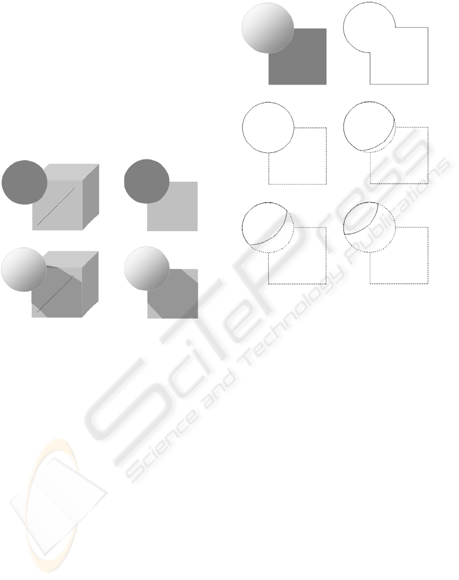
(R.L.Cook and K.E.Torrance, 1982). Figures 1(a) and
(c) show a sphere object O in the scene S with or
without a light source. Thanks to the occlusion and
transparency operations, we obtain images shown in
figure 1 (b) and (d) repectively. The image intensity
for each region depends straight on the characteristics
of the object material, on the light source intensity and
on the view point respective to the object surface and
the light source direction.
(a) (b)
(c) (d)
Figure 1: Image construction :(a) an object in the scene,
(b) an image constructed from (a), (c) the same scene with
light, (d) an image reconstructed from (c).
In the absence of more a priori information about
objects and scenes in images, we assume that objects
are uniform (level sets). Each level set then repre-
sents an object in a scene locally viewed as a binary
image. Yet, the operation used for decompositon is
unknown, then it is stated here that level sets are com-
bined solely by the occlusion operation. Figure 2
shows an example of such decomposition.
Boundaries of level sets are called level-lines L
λ
.
Actually, level-lines do not exist since they are located
between pixels. Objects can combine many regions
but they never overlay. Level-lines from the same
level set do never overlay or cross. But level-lines
from different level sets can overlay of course. Let
these overlayed level-lines for λ from u to v be the
level-line flow, the flow extension E is then defined
by v − u.
F
u,v
= {L
λ
λ ∈]u, v]} (1)
By construction, true occlusions between objects in
the scene reflect on junctions in the image, to be fur-
ther detected by the occlusion operation. These junc-
(a) (b)
(c) (d)
(e) (f)
Figure 2: Image decomposition into level sets : (a) the
sphere image, (b)-(f) level set with different λ.
tions are located at the point, between any four neigh-
bour pixels, where two different level-lines merge or
split. Many junctions appear or disappear from an
image to the other. This phenomenon occurs with
important light changes or noise. We call that type
of junctions the virtual junctions. Their unstability
comes from the fact that they originate in intensity
variations wrt. the same material/surface of an ob-
ject in the scene Conversely, junctions from real oc-
clusions in the scene remain quite stable along with
images. We call real junctions these latter consistent
ones. They are actually produced by the reflectance
of different materials for the same light source. That
is why real junctions are invariant to contrast changes.
Also, they likely correspond to a higher contrast be-
tween regions than virtual junctions’. To distinguish
between real and virtual junctions, we then look for
a repetition of the same junction at a point in the im-
age (overlayed junctions). The more the more likely.
From this property, real junctions thus materialize as
flow junctons where E measures the repetition num-
ber. Junctions can be classified into three types : X
junction formed by three level-line flows, Y junction
formed by two level-line flows and L junction (corner)
formed by one level-line flow. In section 4 we discuss
how to extract Y and L junctions. Real X junctions
VISAPP 2006 - IMAGE ANALYSIS
258

are rare and can be considered Y junctions anyway by
ignoring the smallest flow among four (see section 4).
3 DETECTION OF POTENTIAL
FLOW JUNCTIONS
When extracting flow junctions based solely on the
flow extension threshold E, results turn out to be still
very sentitive to local noise. All the more as it is dif-
ficult to set an appropriate threshold for all conditions
inside an image. Following the argument in the sec-
tion above, E represents a degree of reality for a junc-
tion, and mostly virtual junctions should be sentitive
to contrast changes. For a noise resistant detector, we
first select potential flow junctions by measuring the
variation around junction points (between any four
neighbour pixels). Measures of the variation at a point
were studied by many authors, since pixels around the
singularity show a much higher variation than edge-
or region-pixels . Moravec (Moravec, 1979) deter-
mined the variation by computing various intensity
directionnal differences inside a small window and its
neighbourhood. Harris (Harris and Stephens, 1988)
developed a popular local operator by computing and
diagonalizing the covariance of first order direction-
nal derivatives as an analytic image expansion within
a Gaussian weighted circular window for noise re-
ducing and extension framing. A common problem
with all methods of the kind is that their response
depends considerably on the constrast range. That
makes it difficult to set parameters or thresholds. Ad-
ditionnally many of them use a Gaussian smoothing
to noise reduction that hampers junction localization
as a side effect. From both main problems it did
not seem adequate to adapt such methods to level
lines. Completely different approaches like Girard’s
(Girard, 1980), the one by Bonnin and al. (Bonnin
et al., 1989) or Smith and Brady’s SUSAN (Smith and
Brady, 1997) measure the variation in making no as-
sumption about junction types and without any prior
smoothing. The threshold is simply used as an inten-
sity variation range limit . They assume that junctions
are formed by a couple of regions having constant
or near constant intensity. That makes implicitly the
method limit to L junctions (corners). Here we pro-
pose an extension of SUSAN like methods, adapted
to flow junctions tracking and improved to deal with
other types of junctions.
In the classic SUSAN method, a circular mask is
applied at each pixel p then one measures intensity
variations between p and every other pixel within the
mask. If N
p
is the number of pixels where the vari-
ation is less than a threshold
E
2
and N
p
is less than
half the mask size N
m
the center pixel is considered a
potential junction with response V
p
. The area in the
mask covered by these pixels is called USAN.
N
p
=
p
i
∈w
C
p
i
C
p
i
=
1 if |I(p) − I(p
i
)|≤
E
2
0 else
(2)
V
p
=
N
m
2
−N
p
if N
p
<
N
m
2
0 else
(3)
Adapting the idea to flow junctions, we keep the
same formulas to computing N
p
but we consider that
junction points are located between any four pixels.
We define the flow junction variation V
p
as the sum
of all pixel variations V
p
around that point.
V
p
=
N
m
2
−N
p
if
N
m
16
≤N
p
<
N
m
2
0 else
(4)
N
m
16
is considered as the minimum corresponding to
2 pixels out of 36 (# 22.5 degrees) similar to p. Since
each pixel’s variation marks an L junction, the total
variation shows implicitly the X and Y flow junctions.
The figure 3 displays an example of Y junction. How-
ever this summation is computed under the condition
that the difference between the maximum and min-
imum average intensity of FLAM’s area be greater
than or equal to the flow extension E (FLAM stands
for Flow Laminating Average Milieu and is the geo-
metric equivalent to the Smith’s USAN in the case of
level lines). This difference value indicates the largest
level-line flow that could pass though the junction in
question. The variation at a junction point is thus de-
fined as
V
p
=
i∈[1,4]
V
2
p
i
if M
+
p
−M
−
p
≥E
0 else
(5)
Note that the average intensity for FLAM’s area
M
p
is computed as.
M
p
=
[p
i
∈w|I(p)−I(p
i
)|≤E]
I(p
i
)
N
p
(6)
Then M
+
p
= max(M
p
i
i ∈ [1, 4]) and M
−
p
=
min(M
p
i
i ∈ [1, 4])). The junction variation com-
puted this way makes the junction variation detector.
Figure 4 makes all notations explicit on the sketch
of a Y junction in the I= f (x, y) space.
In the next section, we show how to track flow
junctions all through the image. Successful tracking
makes the actual junctions, giving rise to the acronym
EFLAM that stands for Extended FLAM. Derived
junctions are to be used further as primitives in a
matching process.
EFLAM: A MODEL TO LEVEL-LINE JUNCTION EXTRACTION
259
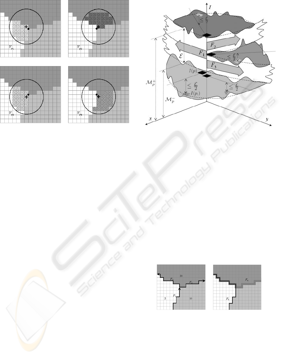
(a) (b)
(c) (d)
Figure 3: FLAM area associated to four pixels around a
junction point and the computed variations. (a) Variation at
pixel p
1
, V
p
1
(b) Variation at pixel p
2
, V
p
2
(c) Variation at
pixel p
3
, V
p
3
(d) Variation at pixel p
4
, V
p
4
.
4 EXTRACTION OF FLOW
JUNCTIONS
Classic methods extract level-line flows in using a
series of thesholds and then follow repetitive over-
layed level-lines from point to point. The method is
straightforward but expensive in terms of computing
time. Here, we propose a tracker automaton that splits
into three main steps.
First step : apply the junction variation detector. It
takes an image for the input and then runs the operator
at every junction point. A positive non zero value is
thus attributed to any potential junction point.
Second step : track level-line flows. For every po-
tential junction point, the automaton tracks level-line
flows that form into it. To that aim, it first determines
the initial flows at that point in the principal directions
according to:
F
i
= {L
λ
λ ∈]u
i
,v
i
]} , i ∈ [1, 4] (7)
Where u
i
= min(M
p
i
, M
p
i+1(mod4)
) and v
i
=
max(M
p
i
, M
p
i+1(mod4)
). Since only Y or L junc-
tions are to be tracked, the antomaton deletes the least
important level-line flows by comparing flow exten-
sions E
i
. Let us underline that E
i
can then make a
control parameter for the density of junctions. Then,
each valid initial flow is tracked through the image in
different directions, following the conditions :
(1) the tracking flow is a subset of the destination
flow,
Figure 4: FLAM area associated to a Y junction.
(2) the tracking path will not return to its origin,
(3) the tracking path favours and preserves straight
lines.
The first condition makes the automaton track
the same level-line flow whatever the local im-
age topology. Conditions (2) and (3) give best
chances to important straight level-line flows in
buffering. The figure 5 (a) shows an example of
level-line flows tracking though a junction where
F
1
= {L
λ
λ ∈]5, 10]} ,F
2
= {L
λ
λ ∈]10, 20]}
and F
3
= {L
λ
λ ∈]5, 20]}. We note that F
1
⊂ F
3
but F
1
F
2
, and F
2
⊂ F
3
but F
2
F
1
, by these
constraints we obtain F
a
= F
2
and F
b
= F
1
that
forms into the junction shown in figure 5(b).
(a) (b)
Figure 5: Level-line flows tracking though a junction.
Third step : code a flow junction as a primitive fea-
ture. At this step the straight level-line flow is ap-
proximated by a segment line. Its descriptors as given
in equation 8 consist of the starting point, the length,
the flow extension, and the average intensities left and
right of the line.
−→
S =[
p E Lc
l
c
r
] (8)
VISAPP 2006 - IMAGE ANALYSIS
260
Where c
l
=
M
p
l
L
, c
r
=
M
p
r
L
and E =
i<L
|M
p
i
r
−M
p
i
l
|
L
. The Y junction which is formed
by two level-line flows is defined as aprimitive
−→
P
combining three segments. Likewise the L junction
can be approximated by two segments. We define the
principal segment
−→
S
∗
of a primitive as the one sup-
ported by the maximal level-line flow among the three
that join at point p in case of a Y. In case of an L it
corresponds to the first detected flow along with the
image scan. Virtual pixel p is the control point of the
primitive to be further matched. Angles θ
l
and θ
r
are
measured from the principal segment to respectively
the one on its left
−→
S
l
, and the other on the right
−→
S
r
.
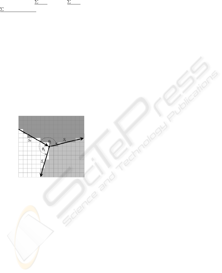
The figure 6 shows the primitive associated to the Y
flow junction in figure 5.
−→
P =
p
−→
S
∗
−→
S
l
−→
S
r
θ
l
θ
r
(9)
Figure 6: Definition of primitive.
Note that binding the principal segment of a prim-
itive to the actual image local configuration makes
flow junctions rotation invariant. Moreover, the order
of magnitude of region intensities around the junction
could constrain the matching tighter.
F
−→
P
= V
p
−→
S
i
∈
−→
P
L
i
×E
i
(10)
F
P
appears eventually as the reliability of a primi-
tive, to be used for non-maximum suppression in the
case we extract corners or for multi-round matching
when primitives would be progressively involved ac-
cording to that latter reliability. Let us underline that,
unlike most methods based on points of interest, no
more descriptor − moment, derivative, Fourier para-
meters etc. − needs to be further computed to match-
ing. Next section starts with comparing our results
to Harris’s, and then stresses upon the control of the
junction scattering over an image.
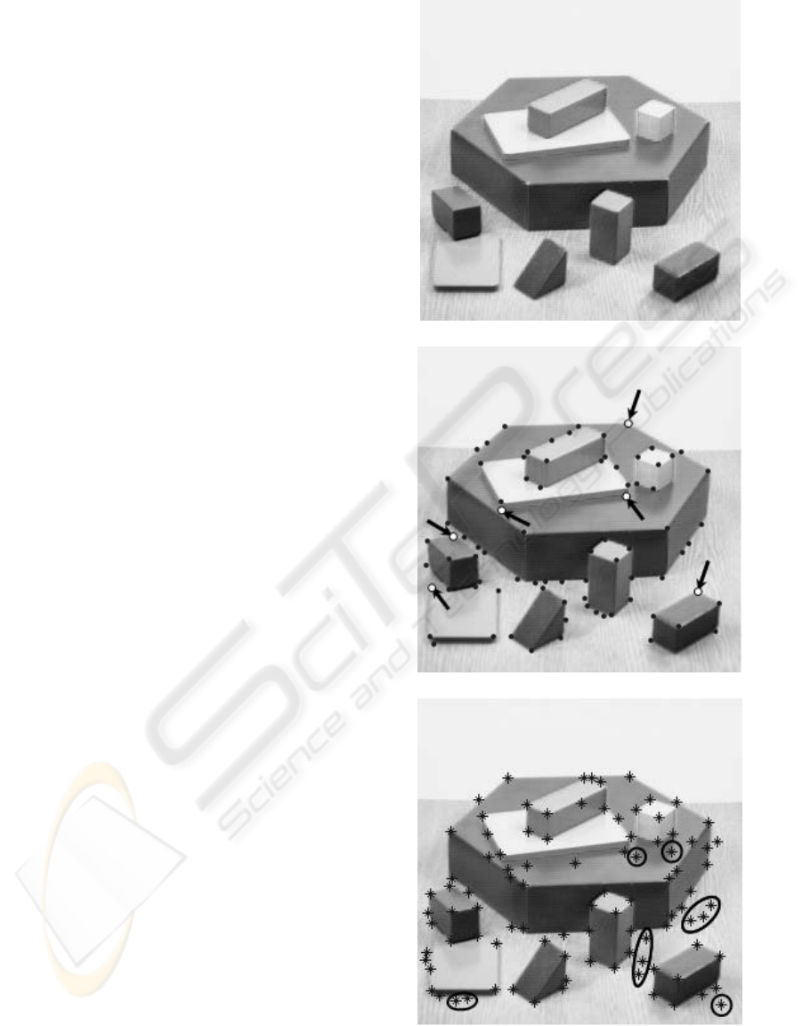
5 RESULTS
The performance of our method is compared to the
one by Harris on real scene images, shown in figure
7(a) ”block image” and figure 10(a) ”house image”.
We select the Harris detector, not SUSAN or others,
for appearing as the more dependable especially with
affine transforms even if it is not the more precise or
robust to noise. The best results of the Harris op-
erator, as found in ”
http://www.cim.mcgill.ca/ dparks/”,
are displayed in figure 7(b) and 10(b) respectively.
By applying our method with E =10, all junctions
extracted from ”block image” before non-maximum
suppression are shown in figure 9(a). Figure 9(b)
displays junctions selected from figure 9(a) as local
maxima by their reliability. Junction points are then
superimposed in ”block image” (figure 7(c)) to com-
pare with the Harris operator. All corners are found
by EFLAM unlike with Harris as indicated by the ar-
rows. This is to the price of more edge-like points.
Our detector is more sensitive to shadows (see cir-
cled points in figure 7(c)). Yet our results are bound
to the selection strategy for E. Increasing E to 14 8,
gets rid of shadow/edge points to the detriment of the
precision of point location. Similarly, by applying
the method to ”house image” all extracted junctions
and sectected junctions are shown in figure 11(a) and
11(b) respectively. Results interpretation remains the
same for 9(b) and (c) as for 7(b) and (c). However
our miss of the upper right corner of the bright verti-
cal window shows the criticity of E , whence the next
kind of experiments about possible loops on E while
matching.
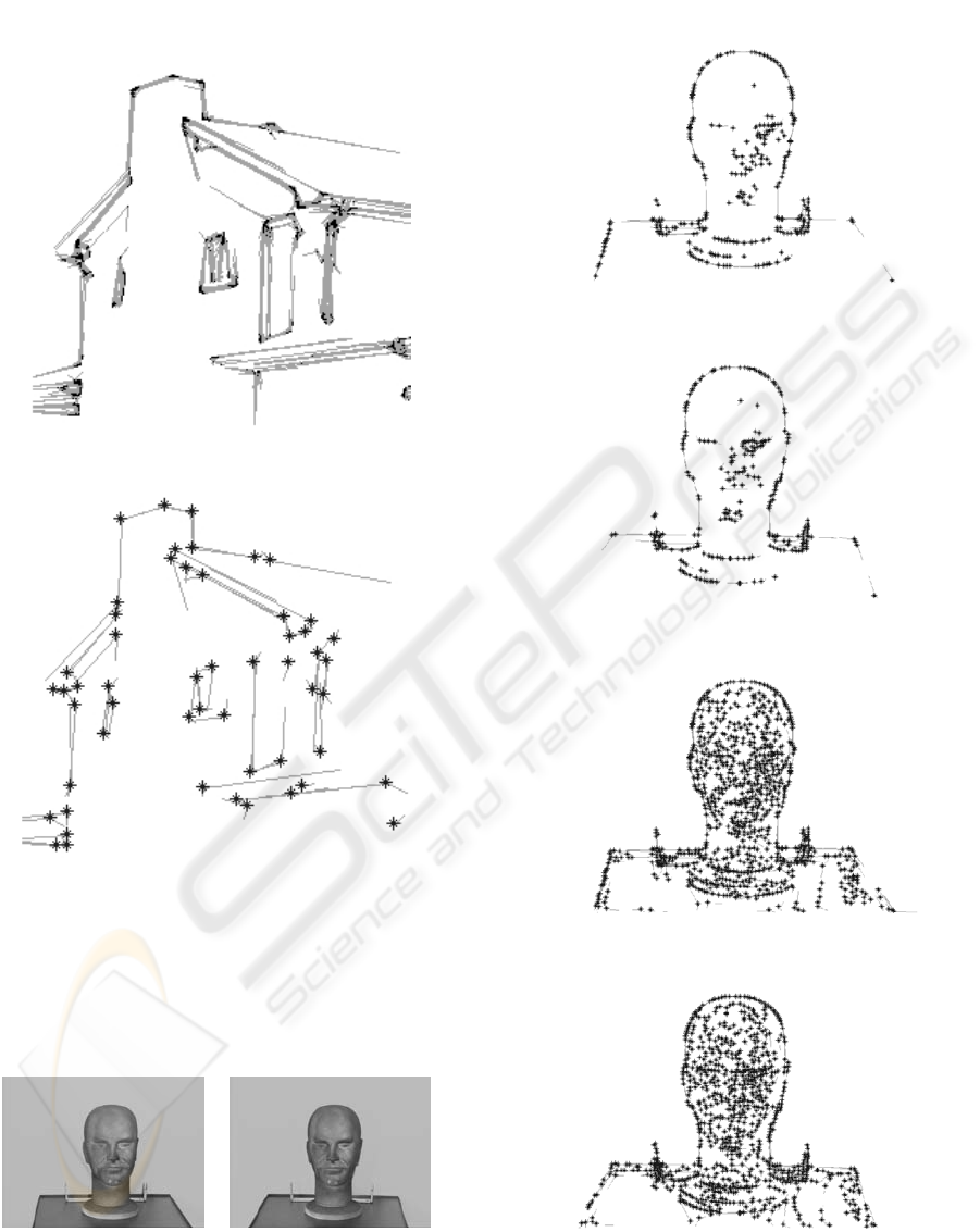
Indeed, another important advantage to stress upon
is that we can control the spread of extracted junc-
tions over the image. That is very important e.g.
for 3D reconstruction. The extraction is performed
as a repetitive process by decreasing the flow exten-
sion E. At the beginning, junctions are extracted with
a high value of E. Then an exclusion zone is de-
fined as a circular area around any extracted junction
point. Next round, the extraction method repeats with
a lesser value of E adding newly found junctions only
in the authorized empty zones. The smaller E, the
more occuring junctions. Note that since the relia-
bility of primitives is computed from the flow exten-
sion E respective to length and variation, primitives
obtained early in the process are likely more reliable.
That turns out to be very useful for multi-round math-
cing.
Figures 12(a) and (b) show an example of ”bust”
stereo images. Extracted junctions from the left and
right images in the first round, where E =20, are
shown in figure 13(a) and (b) respectively. The ex-
tracted junctions cover barely principal structures :
head, eyes, mouth, and nose. Figure 13(c) and (d)
show the second round of extraction, where E =15,
EFLAM: A MODEL TO LEVEL-LINE JUNCTION EXTRACTION
261
adding to junctions extracted from the first round.
Now junctions represent more details of the face,
while being regularly organized that helps reconstruc-
tion..
6 CONCLUSION
We presented in this paper the extraction of level-line
junctions. The method is based on both level-line
flow and flow junction concepts. The potential flow
junctions are first detected according to the EFLAM
model. It computes the variation around any junction
point from the FLAM’s areas. The method makes ex-
tracted junctions robust to noise and contrast change.
The image primitives coded from extracted junctions
are rotation invariant thanks to the local image pat-
tern. One main advantage of our method is that we
can control the spread of extracted junctions over an
image and that is very useful for matching in general
and peculiarly 3D reconstruction.
REFERENCES
Blinn, J. F. (1977). Models of light reflection for com-
puter synthesized pictures. SIGGRAPH’77 Proceed-
ings, 11(2):192–198.
Bonnin, P., Pauchon, E., and Zavidovique, B. (July 1989).
Tracking in infrared imagery based on a point of inter-
est/region cooperative segmentation software agents
activities. In ICIP’89, 3rd International Conference
on Image Processing, Warwick. ICEIS Press.
Caselles, V., Coll, B., and Morel, J.-M. (1999). Topographic
maps and local contrast changes in natural images. Int.
J. Comput. Vision, 33(1):5–27.
Girard, M. (1980). Digital target tracking. In NATO Group,
Aalborg, Denmark.
Harris, C. and Stephens, M. (1988). A combined corner
and edge detector. In Proceedings of The Fourth Alvey
Vision Conference, pages 147–151, Plessey Research
Roke Manor, UK.
Monasse, P. and Guichard, F. (1998). Fast computation of a
contrast-invariant image representation. IEEE Trans.
on Image Proc., 9(5):860–872.
Moravec, H. P. (1979). Visual mapping by a robot rover.
In International Joint Conference on Artificial Intelli-
gence, pages 598–600.
R.L.Cook and K.E.Torrance (1982). A reflectance model
for computer graphics. Transactions on Graphics,
1(1):7–24.
Smith, S. M. and Brady, J. M. (1997). Susan - a new ap-
proach to low level image processing. Int. J. Comput.
Vision, 23(1):45–78.
(a)
(b)
(c)
Figure 7: (a) Block test image (b) Harris corners (c) Corner
by our method, E =10.
VISAPP 2006 - IMAGE ANALYSIS
262
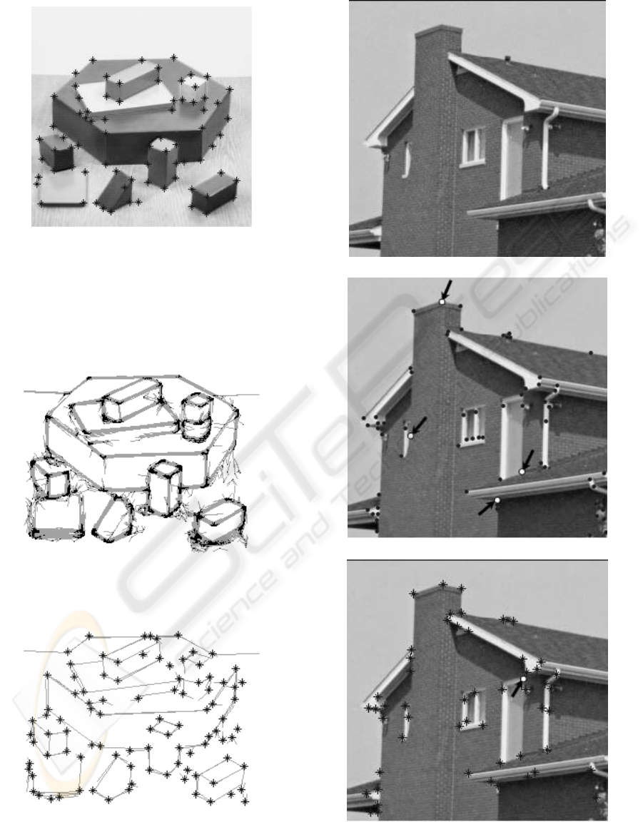
Figure 8: Trade-off between shadow-avoidance and pre-
cision for near optimal corner detection by our method,
E =14.
(a)
(b)
Figure 9: (a) Junctions before filtering, E =10(b) Junc-
tions after filtering, E =10.
(a)
(b)
(c)
Figure 10: (a) House test image (b) Harris corners (b) Cor-
ner by our method with E =30.
EFLAM: A MODEL TO LEVEL-LINE JUNCTION EXTRACTION
263
(a)
(b)
Figure 11: (a) Junctions before filtering, E =30(b) Junc-
tions after filtering, E =30.
(a) (b)
Figure 12: Stereo images (a) left image (b) right image.
(a)
(b)
(c)
(d)
Figure 13: (a) Junctions of left image, E =20(b) Junctions
of right image, E =20(c) Junctions of left image, E =15
(d) Junctions of right image, E =15.
VISAPP 2006 - IMAGE ANALYSIS
264
