A NEUROBIOLOGICALLY INSPIRED VOWEL

RECOGNIZER USING HOUGH-TRANSFORM

A novel approach to auditory image processing

Tamás Harczos

Péter Pázmány Catholic University, Práter Street 50/a, Budapest 1083, Hungary

Frank Klefenz, András Kátai

Fraunhofer Institute for Digital Media Technology, Langewiesener Street 22, Ilmenau 98693, Germany

Keywords: auditory image, Hough-transform, vowel recognition.

Abstract: Many pattern recognition problems can be solved by mapping the input data into an n-dimensional feature

space in which a vector indicates a set of attributes. One powerful pattern recognition method is the Hough-

transform, which is usually applied to detect specific curves or shapes in digital pictures. In this paper the

Hough-transform is applied to the time series data of neurotransmitter vesicle releases of an auditory model.

Practical vowel recognition of different speakers with the help of this transform is investigated and the

findings are discussed.

1 INTRODUCTION

Vowel recognition is a wide research area with

many existing solutions. The authors will now

present a method how a standard image processing

algorithm like the Hough-transform can be applied

to process audio signals. The time-varying audio

signal is first transformed by a neurophysiologically

parameterized Extended Zwicker / Meddis-Poveda

auditory model into a two-dimensional

spatiotemporal neurotransmitter vesicle release

distribution. The Hough-transform is then applied to

this image to detect the emerging vesicle release

patterns evoked by vowels.

1.1 The Hough-transform

The Hough-transform is a technique that can be used

to isolate features of a particular shape within an

image (Shapiro, 1978). It was originally developed

in the field of high-energy physics for the detection

of charged particle tracks in bubble chambers to

detect straight lines (Hough, 1959), (Hough, 1962).

Since then it has been used as a standard image

analysis tool for pattern recognition, and has been

generalized to arbitrary shapes (Duda, 1972),

(Ballard, 1981). The procedure has similarities to

regression methods, the common problem being to

derive line parameters from points lying on that line

(Ohlsson, 1992). The Hough-transform is very

robust; points that are not on the line have little

influence on the estimation. The main advantage of

the technique is that it is tolerant of gaps in feature

boundary descriptions and is relatively unaffected by

image noise.

Hough-transform is a coordinate transform,

which maps the input data directly to an n-

dimensional feature space, in which the aggregating

clusters indicate the occurrence of a feature. The

attributes of a feature are quantitatively coded by the

corresponding n-dimensional feature vector. The

feature attributes are mapped linearly along the

orthogonal feature axes. The power of the Hough-

transform derives from the linearity of the feature

maps.

Input tuple coordinates and feature coordinates

are coupled by the corresponding Hough-transform

equations (Duda, 1972). These equations can be

given analytically for simple patterns like straight

lines, circles and trigonometric functions (Ballard,

1981). Each input tuple is translated to its associated

trajectory in the corresponding feature space.

Multiple crossings of trajectories in the feature space

indicate that a feature forming input tuple set

belongs to the same feature. The multiple

intersections of the trajectories lead to clustering in

the feature space. However, the intersection density

peaks sharply for the best possible fit of an observed

feature, therefore a single feature is represented in

251

Harczos T., Klefenz F. and Kátai A. (2006).

A NEUROBIOLOGICALLY INSPIRED VOWEL RECOGNIZER USING HOUGH-TRANSFORM - A novel approach to auditory image processing.

In Proceedings of the First International Conference on Computer Vision Theory and Applications, pages 251-256

DOI: 10.5220/0001363902510256

 SciTePress

the feature space as a point distribution with

characteristic decreasing profile (Davis, 1992).

1.2 Parallel Hough-transform

The Hough-transform algorithm is known to be

computational intensive (Swaaij, 1990). In the dis-

crete form, it is a histogram accumulating technique.

The feature space is subdivided into a grid of histo-

gram cells, whose number defines the granularity of

the feature space. The Hough-transform is therefore,

in its discrete form, a histogram updating procedure

in which for each point (or event) in the input data,

we update the histogram in the Hough space. The

result is a 2-D histogram representing for each point

in the parameter (Hough) space, the probability of

the existence of a shape with such parameters.

Hubel et al. (Hubel, 1978) demonstrated the

natural orientation columns in the macaque monkey

brain, which are believed to perform a kind of

parallel Hough-transform, serving the orientation of

the monkey by extracting features from the seen

image in real-time. One can easily come to the idea

of trying to model this naturally brilliant

architecture, hoping that the same speed-up can be

achieved.

Epstein et al. (Epstein, 2001) designed a parallel

Hough-transform engine, where, in reducing the n-

dimensional feature space to two dimensions the

coordinate transform can be executed by a systolic

array consisting of time-delay processing elements

and adders.

1.3 Application to sound data

Generally speaking, sound is an oscillation of air

pressure level in time. To process a piece of sound in

a digital system, it first has to be digitized. The

monoaural sounds that we use in this project are

recorded with a sampling rate of 44.1 kHz and a

resolution of 16 bits. Due to some similarity between

pattern recognition and statistical curve fitting

problems, the Hough-transform may as well be

directly applied to digitized sound data. The direct

appliance to the time varying audio signal is

discussed by Röver et al. for musical instrument

identification (Röver, 2004). Brückmann et al. have

shown that not only video signals as bars of different

slopes, but also audio signals as sinusoids are self-

learned by feed-forward timing neural networks.

These nets learn the Hough-transform in most of the

cases (Brückmann, 2004).

2 MOTIVATION: DELAY

TRAJECTORIES

The application of the Hough-transform to the

output of an auditory model is motivated by the fact,

that a sound might be represented by regular shapes

in an intermediate representation, which might be

identifiable by the Hough-transform. We choose the

neurotransmitter release distribution as the inter-

mediate input for the Hough-transform. The patterns

of the neurotransmitter concentration in the synaptic

cleft have the appearance to be bundles of curves of

different curvature, if quasi stationary signals such

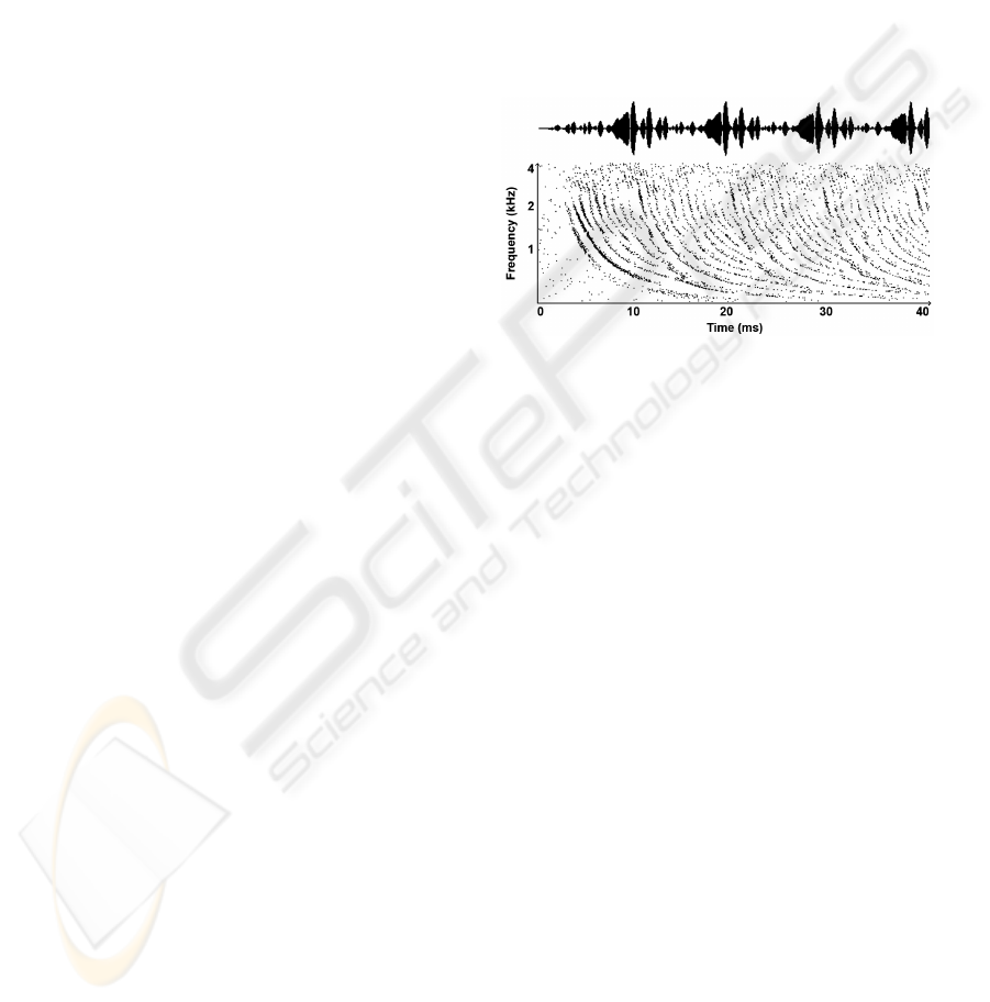
as vowels are applied (see Figure 1).

Figure 1: waveform (top) and vesicle release delay

trajectories (bottom) of vowel "a" (male speaker).

According to the auditory image (AI) study from

Greenberg et al. (Greenberg, 1997) the curvature of

the resulting curve caused by a single impulse is

solely dependent on the species, i.e., the anatomical

properties of the basilar membrane (BM). On the

other hand, when speaking of one species and

complex sounds, then the resulting curves do have

different curvature. We concentrate on these

emerging vesicle data sets. We will try to detect

these emerging curves composed of vesicles by

fitting appropriate curves to the neurotransmitter

vesicle release distribution, and then see whether a

sound can be classified by the generated sequence of

curve parameters. The curve parameters are the time

of occurrence and their specific curvature. The

Hough-transform is then applied to the auditory

image of vowel sounds intonated by different

speakers.

3 THE AUDITORY MODEL

The velocity of the basilar membrane excited by a

time varying audio signal is computed according to

the Extended Zwicker model as given by Baumgarte

(Baumgarte, 2000). The mechano-chemical coupling

of the BM velocity is mediated by the forced

movement of the stereociliae of the inner hair cells

(IHC). The movement depolarizes the IHCs

resulting in neurotransmitter vesicle releases. This

VISAPP 2006 - IMAGE ANALYSIS

252

process is modelled according to the rate kinetics

equations as given by Meddis and Poveda in

(Sumner, 2002). The neurotransmitter release

distribution reflects the actual state of the BM

velocity at a given time.

The auditory model processes the wave input file

and generates 251-channel output data, where each

channel has a different centre frequency, ranging

from 5 Hz to 21 kHz. The channels can be imagined

as slices of the basilar membrane in the cochlea with

the data on them representing the sound information

sent by the inner hair cells towards the brain.

4 CORE: THE NEURAL NET

The core of the system is an artificial Hubel-Wiesel

network, which is extensively described in

(Brückmann, 2002). This neural network is able to

learn almost any set of different slopes or a set of

sinusoids of different frequencies. It has been also

shown, that the network is capable of self-learning,

however, this process may consume large amount of

time.

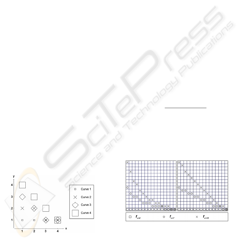
Katzmann showed (see Acknowledgements) that

a more efficient learning method is available if the

following rules are satisfied (see also Figure 2):

- the curves (to be taught) must be one pixel

wide,

- for every x-value a function value (a pixel of the

curve) must exist,

- the first “curve” should always be a straight

horizontal line (y=1),

- the curves should be ordered by an index, where

the (i+1)

curve must be at most one pixel

wider (in y direction) than the i

one,

- all curves must start at first column (x=1) and

go down to the rightmost, lowest point (x

last

, y=1).

Figure 2: a 4x4 network with four possible curves.

Please note that the curves created according to the

method defined above will be inverted before use,

i.e., the first curve being looked for in the auditory

image will be a straight vertical line.

5 PARAMETERIZATION

To achieve a good performance, it is crucial to have

the proper curves modelled and to do the Hough-

transform on the appropriate data set.

5.1 Geometric model of the curves

Greenberg pointed out that the motion of the BM

proceeds in an orderly fashion from the base to the

point of maximum displacement, beyond which it

damps out relatively quickly. The transit of the

travelling wave is extremely fast at the base, but

slowing dramatically for peak displacements at the

apex of the cochlea (Greenberg, 1997). He showed,

furthermore, that the delay trajectories can be

efficiently modelled by the simple equation:

kfd

−1

, (1)

where the cochlear delay d

can be calculated from

the given frequency f

and delay constant k.

Basically, the equation above means that the delay

trajectories have some kind of 1/x characteristics.

Based on this statement, and taking the rules

listed in Chapter 4 into account, we found the

following curve-equation for our digital system:

)1()(

)1(

)(

min

−⋅+

−−⋅

⋅

nfj

jnf

, (2)

where n

is the size of the quadratic network in each

direction (measured in pixels), ν denotes the index of

the current curve (ν= 0, 1, …, n

–

1), and j is the

index of the current pixel being calculated (j= 0, 1,

…, n

–

1). Free variable f

min

can be used to set the

average curvature, see Figure 3 for comparison.

Figure 3: 16x16 networks configured with different f

min

value (left: f

min

= 5, right: f

min

= 35). Note that only 3 of the

16 curves are shown on each figure.

5.2 Hough parameters

As already mentioned in the introductory part, the

extraction of the curves is performed by an artificial

Hubel-Wiesel network in a parallel way. Parallel

A NEUROBIOLOGICALLY INSPIRED VOWEL RECOGNIZER USING HOUGH-TRANSFORM - A novel approach to

auditory image processing

253

operation stands for a line-wise instead of a pixel-

wise approach.

As stated in Chapter 3, our auditory model has

251 channels of output, each corresponding to a

specific centre frequency. Since speech processing

does not require the whole spectral information, a

spectral crop can be applied to decrease the number

of channels to be processed. We now introduce two

new system parameters: C

and C

, which stand for

bottom- and top (spectral) crop, respectively. Both

are non-negative integers and mean the number of

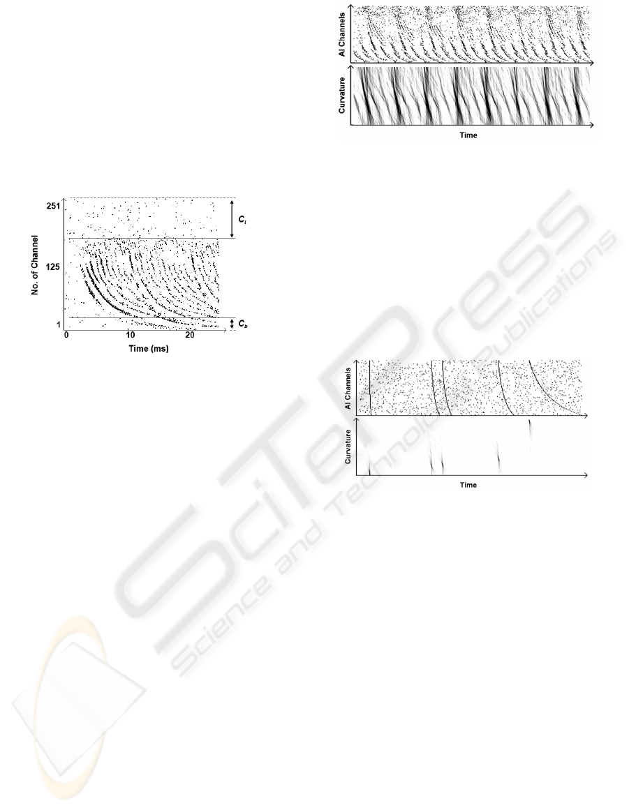
channels to be ignored (see Figure 4).

Figure 4: cropping of the auditory image.

One other system parameter is S

, which stands for

time-scaling. S

is the number of consecutive data on

each channel, which will be averaged and treated as

one input data for the Hough-transform.

So, the main parameter quadruplet for the

Hough-transform is f

min

, C

and S

. The best

values are different for men and women voice, but

min

= 30, C

=25, C

=85 and S

=6 is a good

compromise. From now on, these values will be

referred as the default Hough parameters.

It is easy to see, that the height of the auditory

image to be transformed, and hence, the size of the

artificial Hubel-Wiesel network is h=251–C

–C

The width (w) of the image depends on the duration

of the input sound and on S

6 THE TRANSFORMATION

Once the input sound file has been transformed into

an auditory image, the Hubel-Wiesel network will

be configured, i.e., the curves corresponding to a

given f

min

will be taught.

Next, the cropped auditory image will be fed into

the network. In each step, the image will be shifted

by one column that the network will transform. Each

step generates an output array of h elements. Since

our artificial Hubel-Wiesel network is quadratic, in

w steps, the Hough-transformed output image

(having the same dimension as that of the input

image) will be ready.

Figure 5: delay trajectories of (male) vowel “e” induced

by the highly coherent neurotransmitter vesicle releases

(top), and its Hough-transformed image (bottom).

If the Hough parameters were set correctly, the

output image would give clear information about

“when” and “what curvature” curves were contained

by the auditory image (see Figure 5 and Figure 6).

For better understanding, see Figure 6, where a

fake auditory image with five artificially created

curves has been overlaid with random noise and then

transformed. Note that the transformed output image

(bottom) only contains five distinctly visible points

representing the five original curves (top).

Figure 6: a Hough-transformed fake auditory image.

7 RECOGNITION

To achieve a clear transformed image (similar to

Figure 6, bottom), and to enable an experimental

vowel recognition, the Hough-transformed auditory

image (AI) has to be post-processed. A typical post-

processing step for Hough-transform is the so called

butterfly filtering, which is a convolution filter, and

is used to enhance the feature points in the

transformed image. Still, since we only need several

feature points for vowel recognition we chose

another way of post-processing as follows.

7.1 Post-processing

The (greyscale) value for each pixel in the

transformed image ranges from 0 to h-1. Let us

denote the x and y position and the value of the

global maximum pixel by m

, m

and m

, respec-

tively. Furthermore, the pixels of the transformed

image will be referred as P

x,y

, where, for example,

5,8

means the value of the pixel that is the 5

from

VISAPP 2006 - IMAGE ANALYSIS

254

the left and the 8

from the bottom of the image.

Now, histogram H

will be built according to the

pixel values of all the rows of the transformed image

(see Equation 3 and Equation 4). H

will contain the

sum of those pixel-values in a line, which are greater

or equal to τּ m

. Default value for τ is 0.75.

⎪

⎩

⎪

⎨

⎧

⋅≥

otherwise

mPP

yxP

vyxyx

),(

(3)

∑

yiPyH

),()(

ττ

(4)

Now, let smooth H

and take the positions of the

three major peaks; denote them by Φ

(highest

peak), Φ

and Φ

(smallest peak). Taking the peak

values from the histogram will determine the y

position of the areas, in which an adaptive (local)

maximum search shall be initiated. The x position of

the search areas will be determined by calculating

the highest autocorrelation value (ρ: best

periodicity) of the transformed image, and by adding

this ρ several times to the x position of the

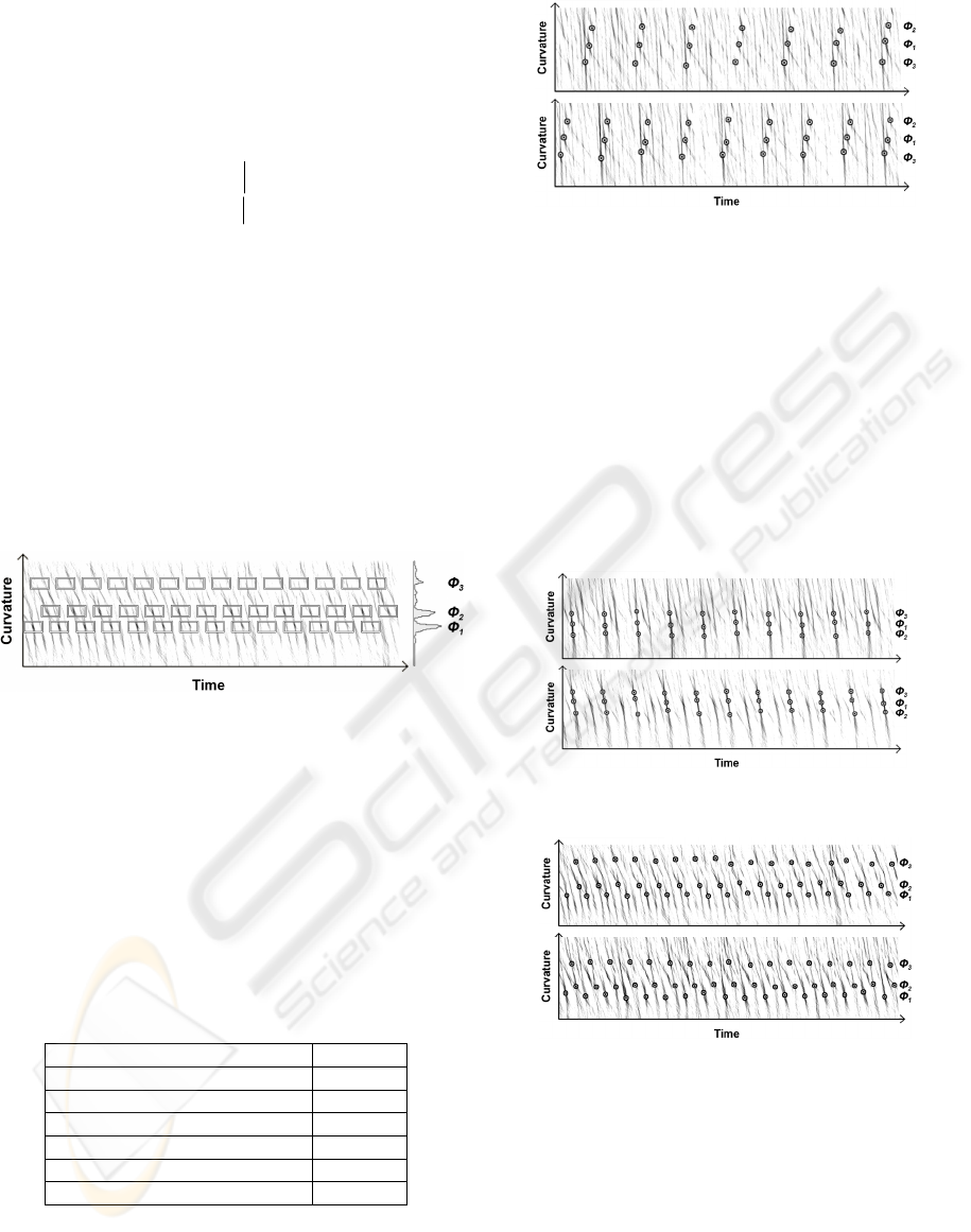
maximum pixel in the actual line (see Figure 7).

Figure 7. Hough transformed AI of vowel “u” (female

speaker). The local-maximum (LM) search-areas

(boxes) based on the histogram (right) are also shown.

Please note the order of Φ

, Φ

and Φ

, and that ρ

equals to the displacement between adjacent boxes.

7.2 The resulting data set

Quadruplet [Φ

, Φ

, ρ] contains sufficient

information to carry out a simple vowel recognition.

We introduce a redundant variable r for easier

discussion of the relation of the histogram peaks (see

Table 1).

Table 1: Possible relation of histogram peaks.

Relation of peak positions

< Φ

We state that efficient and robust automated vowel

recognition might be possible based on H

and ρ.

Figure 8: Hough-transformed AIs of vowel “a”, with the

maximum points (of LM-areas) shown. Top: male speaker

A, bottom: male speaker B. Please note the similarities,

and the fact that in both cases r=5 holds.

7.3 A simple recognition method

As the next step of a very simple vowel recognition

and visualization procedure, the maximum value of

each LM-area (see boxes on Figure 7) will be

picked. Then, based on the histogram, r will be

evaluated. Most amazingly, r itself is a very strong

feature for vowels “a”, “o” and “u”, even for

different speakers. See Figure 8, Figure 9 and Figure

10 for comparison.

Figure 9: Hough-transformed AIs of vowel “o”, with the

maximum points shown. Top: male speaker B, bottom:

male speaker C. In both cases r=3 holds.

Figure 10: Hough-transformed AIs of vowel “u”, with

the maximum points shown. Top: female speaker A,

bottom: female speaker B. In both cases r=1 holds.

The results presented above are very similar in the

case of other speakers.

7.4 Visualization of the results

One could doubt whether the maximum points

would be found correctly. The maximum points can

be picked and the curves that they encode can be

drawn back for verification. See Figure 11. The

results do not need any further explanation.

A NEUROBIOLOGICALLY INSPIRED VOWEL RECOGNIZER USING HOUGH-TRANSFORM - A novel approach to

auditory image processing

255

Figure 11: Hough-transformed AI of vowel “i” by male

speaker B with maximum points shown (bottom), and the

corresponding delay trajectories with curves drawn back

based on maximum point information (top). Please note

that despite the similarity to Figure 8, r=2 in this case.

8 RESULTS

It has been shown that after the Hough-transfor-

mation of the auditory image, vowels can be recog-

nized even with very simple processing methods.

Despite the simplicity of the algorithm, recognition

is speaker-independent for selected vowels (a, o, u).

We insist that a competent (neural) system could do

a more extensive and yet robust recognition based

on H

and ρ.

9 CONCLUSIONS

The application of the Hough-transform to the

neurotransmitter vesicle release distribution yields

good results, especially in procuring invariant

parameter settings for vowel descriptions for

different speakers. According to these findings, the

authors will try to model several computational

maps in the brain structured to execute Hough-

transforms. Furthermore, more sophisticated post-

processing methods are being investigated to yield a

more robust and possibly automated vowel

recognition.

ACKNOWLEDGEMENTS

We acknowledge the help of and would like to thank

Johannes Katzmann for his efficient Hubel-Wiesel

learning method (Katzmann, 2005), Andreas

Brückmann for the Hubel-Wiesel network

configuration program, and Gero Szepannek for the

stochastic modelling of the IHCs.

REFERENCES

Shapiro, S.D., 1978. Feature Space Transforms for Curve

Detection. Pattern Recognition, 10, pp 129–143.

Hough, P.V.C., 1959. Machine analysis of bubble

chamber pictures. Proceedings of the International

Conference on High-Energy Accelerators and

Instrumentation, L. Kowarski (Editor), CERN, pp

554–556.

Hough, P.V.C., 1962. Method and means for recognizing

complex patterns. US Patent 3069654.

Duda, E.O., Hart, P.E., 1972. Use of the Hough transform

to detect lines and curves in pictures. Comm. ACM, pp

11–15.

Ballard, D.H., 1981. Generalizing the Hough transform to

detect arbitrary shapes. Pattern Recognition 13, pp

111–122.

Ohlsson, M., Peterson, C., Yuille, A.L., 1992. Track

finding with deformable templates - the elastic arms

approach. Comp. Phys. Comm. vol. 71, pp 77–98.

Davis, E.R., 1992. Modelling peak shapes obtained by

Hough transform, IEEE proceedings vol. 139, 1.

Swaaij, M. Van, Catthoor, F., De Man, H., 1990. Deriving

ASIC architectures for the Hough transform. Parallel

Computing 16, pp 113–121.

Hubel, D.H., Wiesel, T.N., Stryker, M.P., 1978.

Anatomical demonstration of orientation columns in

macaque monkey. Journal of Comparative Neurology

177, pp 361–380.

Epstein, A., Paul, G.U., Vettermann, B., Boulin, C.,

Klefenz., F., 2001. A parallel systolic array ASIC for

real time execution of the Hough-transform. E. S.

Peris, A. F. Soria, V. G. Millan (Editors). Proceedings

of the 12th IEEE International Congress on Real Time

for Nuclear and Plasma Sciences, Valencia, pp 68–72.

Röver, Ch., Klefenz, F., Weihs, C., 2004. Identification of

musical Instruments by Means of the Hough

Transform. C. Weihs, W. Gaul (Editors). Proceedings

of the 28

Annual Conference of the Gesellschaft für

Klassifikation e. V., University of Dortmund, pp 608–

615.

Brückmann, A., Klefenz, F., Wünsche, A., 2004. A

neural net for 2d-slope and sinusoidal shape detection.

Int. Scient. J. of Computing 3 (1), pp 21–26.

Greenberg, S., Poeppel, D., Roberts, T., 1997. A Space-

Time Theory of Pitch and Timbre Based on Cortical

Expansion of the Cochlear Traveling Wave Delay.

Proceedings of the XI

Int. Symp. on Hearing,

Grantham.

Baumgarte, F., 2000. Ein psychophysiologisches Gehör-

modell zur Nachbildung von Wahrnehmungs-

schwellen für die Audiocodierung. Doctor Thesis,

University of Hannover, Germany.

Sumner, C.J., O'Mard, L.P., Lopez-Poveda, E.A. and

Meddis, R., 2002. A revised model of the inner-hair

cell and auditory nerve complex. Journal of the

Acoustical Society of America, 111, pp 2178–2189.

Katzmann, J., 2005. Echtzeitfähige, auf der Hough-

Transformation basierende Methoden der

Bildverarbeitung zur Detektion von Ellipsen. Diploma

Thesis, University of Ilmenau, Germany.

VISAPP 2006 - IMAGE ANALYSIS

256