
CONSTRAINED GENERALISED PRINCIPAL COMPONENT
ANALYSIS
Wojciech Chojnacki, Anton van den Hengel, Michael J. Brooks
School of Computer Science, University of Adelaide
Adelaide, SA 5005, Australia
Keywords:
Generalised principal component analysis, constrained minimisation, multi-line fitting, degenerate conic.
Abstract:
Generalised Principal Component Analysis (GPCA) is a recently devised technique for fitting a multi-
component, piecewise-linear structure to data that has found strong utility in computer vision. Unlike other
methods which intertwine the processes of estimating structure components and segmenting data points into
clusters associated with putative components, GPCA estimates a multi-component structure with no recourse
to data clustering. The standard GPCA algorithm searches for an estimate by minimising an appropriate misfit
function. The underlying constraints on the model parameters are ignored. Here we promote a variant of
GPCA that incorporates the parameter constraints and exploits constrained rather than unconstrained minimi-
sation of the error function. The output of any GPCA algorithm hardly ever perfectly satisfies the parameter
constraints. Our new version of GPCA greatly facilitates the final correction of the algorithm output to satisfy
perfectly the constraints, making this step less prone to error in the presence of noise. The method is applied
to the example problem of fitting a pair of lines to noisy image points, but has potential for use in more general
multi-component structure fitting in computer vision.
1 INTRODUCTION
One of the challenges of image analysis and com-
puter vision is to develop effective ways to fit a
multi-component structure to data. A classical ex-
ample problem is fitting multiple lines to data (Lou
et al., 1997; Venkateswar and Chellappa, 1992). Sev-
eral methods have been proposed for solving this
particular task, including those based on the Hough
transform (Duda and Hart, 1972), K-subspaces (Ho
et al., 2003), subspace growing and subspace se-
lection (Leonardis et al., 2002), EM (Tipping and
Bishop, 1999) and RANSAC (Forsyth and Ponce,
2003) algorithms. More recently, there has been in-
terest in fitting multiple linear manifolds to data. This
more general problem arose in the analysis of dynam-
ical scenes in computer vision in connection with the
recovery of multiple motion models from image data
(Vidal et al., 2002; Vidal and Ma, 2004; Vidal et al.,
2006). To tackle it, a new approach has been put
forth under the label of generalised principle compo-
nent analysis (GPCA) (Vidal et al., 2003; Vidal et al.,
2004; Vidal et al., 2005). The GPCA method employs
a parametric model in which parameters describe a
multi-component, piecewise-linear structure to which
various parts of a data set adhere. The number of lin-
ear components is assumed to be fixed and known be-
forehand. The relationship between data and compo-
nents is encoded in a multivariate polynomial. In the
special, but representative, case of multi-line fitting,
the components are lines, the order of the polynomial
coincides with the number of the components, and the
recovery of the components is achieved by factoring
the polynomial into a product of multivariate mono-
mials, each corresponding to a separate line. The suc-
cess of the whole procedure rests upon generation of
a meaningful polynomial to factor.
This paper presents a variant of GPCA which ad-
vocates the use of constrained optimisation as a cru-
cial step in component recovery. We concentrate on
a particular problem of fitting two lines to data as in
this case the underlying analysis is particularly simple
and illuminating. Notwithstanding the specificity of
our presentation, the multi-line and, more generally,
multi-component fitting problems can be treated—
upon suitable modification—within the same general
framework.
At the technical level, the contribution of the pa-
per is three-fold. First, it gives a statistically sound
cost function measuring how well a given model in-
206
Chojnacki W., van den Hengel A. and J. Brooks M. (2006).
CONSTRAINED GENERALISED PRINCIPAL COMPONENT ANALYSIS.
In Proceedings of the First International Conference on Computer Vision Theory and Applications, pages 206-212
DOI: 10.5220/0001362102060212
Copyright
c
SciTePress

stance describes the data. The cost function is evolved
by applying the maximum likelihood principle to a
Gaussian model of errors in the data. Second, a pair of
lines is shown to be effectively estimated by minimis-
ing the cost function subject to a certain parameter
constraint. A novel iterative method for computing an
approximate constrained minimiser is given. Finally,
a simple method is presented for converting nearly
optimal estimates obtained by iterative constrained
optimisation techniques (hyperbolae with high eccen-
tricity) into estimates representing a correct geomet-
ric structure (pairs of lines).
The original GPCA algorithm (Vidal et al., 2003;
Vidal et al., 2006) employs algebraic factorisation of
a multivariate polynomial whose coefficients are ob-
tained via unconstrained minimisation of a cost func-
tion equivalent to the one used in the present paper.
The method does not require data segmentation and as
such differs from iterative methods like K-subspaces
and EM which alternate between estimating structure
components and grouping the data around individ-
ual components. However, because of its reliance on
computation of roots of polynomials—a numerically
fragile operation—the GPCA algorithm is sensitive to
noise. To curb adverse effectsof noise, the subsequent
version of GPCA (Vidal et al., 2004; Vidal and Ma,
2004; Vidal et al., 2005) uses polynomial differenti-
ation instead of polynomial factorisation, but at the
cost of employing some form of data segmentation—
one data point per component is needed to effectuate
the estimation step.
The present paper shows—and this is its main con-
ceptual contribution—that the approach taken by the
original version of GPCA can be sustained even in the
presence of moderate noise if unconstrained minimi-
sation is replaced by constrained minimisation. We
demonstrate empirically that constrained optimisation
leads, in practice, to estimates that can be encoded
into nearly factorisable polynomials. These estimates
can be upgraded to estimates corresponding to per-
fectly factorisable polynomials by means of a simple
correction procedure. Because a minor adjustment of
the unconstrained minimiser is needed, the upgrad-
ing procedure operates reliably. Rather than use poly-
nomial factorisation, the correction procedure in our
version of the GPCA involves singular value decom-
position. Its simple form reflects the special nature of
the estimation problem considered.
The estimate obtained by applying the method pre-
sented in the paper represents a pair of lines and as
such is an instance of a conic—a degenerate conic.
Thus, effectively, our variant of GPCA is a method
for degenerate-conic fitting and can be viewed as an
addition to the growing body of algorithms for fitting
to data a conic of a type specified in advance (Fitzgib-
bon et al., 1999; Hal
´
ı
ˇ
r and Flusser, 1998; Nievergelt,
2004; O’Leary and Zsombor-Murray, 2004).
2 BACKGROUND
A line is a focus of points x =[m
1
,m
2
]
T
in the
Euclidean plane R
2
satisfying the equation
l
1
m
1
+ l
2
m
2
+ l
3
=0.
Employing homogeneous coordinates m =
[m
1
,m
2
, 1]
T
and l =[l
1
,l
2
,l
3
]
T
, the same line
can be identified with the subset of the projective
plane P
2
given by Z
l
= {m ∈ P
2
| l
T
m =0}. A
conic is a locus of points x =[m
1
,m
2
]
T
satisfying
the equation
am
2
1
+ bm
1
m
2
+ cm
2
2
+ dm
1
+ em
2
+ f =0,
where a, b and c are not all zero. Introducing the sym-
metric matrix C
C =
ab/2 d/2
b/2 ce/2
d/2 e/2 f
,
the same conic can be described as Z
C
= {m ∈
P
2
| m
T
Cm =0}. A non-degenerate conic satis-
fies det C =0and is either an ellipse, or a parabola,
or a hyperbola depending on whether the discrimi-
nant ∆=b
2
− 4ac is negative, zero or positive. If
det C =0, then the conic is degenerate. A degen-
erate conic represents either two intersecting lines, a
(double) line, or a point, as we now critically recall.
A union of two lines, Z
l
1
∪ Z
l
2
, obeys
l
T
1
m · l
T
2
m = m
T
l
1
l
T
2
m =0
or equivalently, given that m
T
l
1
l
T
2
m = m
T
l
2
l
T
1
m,
m
T
(l
1
l
T
2
+ l
2
l
T
1
)m =0. (1)
With C = l
1
l
T
2
+l
2
l
T
1
, a symmetric matrix, the above
equation can be rewritten as m
T
Cm =0, showing
that Z
l
1
∪ Z
l
2
is identical with the conic Z
C
. The
matrices l
i
l
T
j
are rank-1, so the rank of C is no greater
than 2 and the conic is degenerate. If l
1
= l
2
, then
Z
C
represents a single, repeated line; in this case the
conic equation (l
T
1
m)
2
=0is equivalent to the line
equation l
T
1
m =0. Finally, a point [p
1
,p
2
]
T
can
be represented as the degenerate conic (m
1
− p
1
)
2
+
(m
2
− p
2
)
2
=0corresponding to
C =
⎡
⎣
10−p
1
01−p
2
−p
1
−p
2
p
2
1
+ p
2
2
⎤
⎦
.
To see that a pair of lines, a double line and a point
are the only possible types of degenerate conic, sup-
pose that C is a non-zero symmetric singular matrix.
Then C admits an eigenvalue decomposition (EVD)
of the form C = VDV
T
, where V is an orthogo-
nal 3 × 3 matrix and D = diag(λ
1
,λ
2
,λ
3
), with λ
i
CONSTRAINED GENERALISED PRINCIPAL COMPONENT ANALYSIS
207

(i =1, 2, 3) a real number (Horn and Johnson, 1985).
The eigenvalue decomposition differs from the singu-
lar value decomposition (SVD) of C in that the lat-
ter uses two orthogonal, possibly different, matrices
U and V , and that the former uses a diagonal ma-
trix whose entries are not necessarily non-negative.
However, the EVD and SVD of the symmetric C are
closely related—any of the two orthogonal factors U ,
V in the SVD can serve as V in the EVD, and D in
the EVD can be obtained from the diagonal factor in
the SVD by placing a minus sign before each diago-
nal entry for which the corresponding columns in U
and V differ by a sign, with all remaining entries left
intact. For each i =1, 2, 3, let v
i
be the ith column
vector of V . Then, clearly, v
i
is an eigenvector of
C corresponding to the eigenvalue λ
i
, Cv
i
= λ
i
v
i
,
and, moreover, C =
3
i=1
λ
i
v
i
v
T
i
. Now det C =
λ
1
λ
2
λ
3
=0so one eigenvalue, say λ
3
, is zero, im-
plying that C =
2
i=1
λ
i
v
i
v
T
i
. If another eigenvalue,
say λ
2
, is zero too, then C = λ
1
v
1
v
T
1
and, since
the remaining eigenvalue, λ
1
, has to be non-zero, Z
C
coincides with the line Z
v
1
.Ifλ
3
is the only zero
eigenvalue, then there are two possibilities—either λ
1
and λ
2
are of same sign, or λ
1
and λ
2
are of opposite
sign. In the first case Z
C
reduces to the linear span
of v
3
=[v
13
,v
23
,v
33
]
T
and represents a single point
in P
2
;ifv
33
=0, then this point is part of R
2
and
is given by [v
13
/v
33
,v
23
/v
33
, 1]
T
. In the other case,
Z
C
represents a pair of lines in P
2
. Indeed, without
loss of generality, we may suppose that λ
1
> 0 and
λ
2
< 0. Then
λ
1
v
1
v
T
1
+ λ
2
v
2
v
T
2
= l
1
l
T
2
+ l
2
l
T
1
,
where l
1
=
√
λ
1
v
1
+
√
−λ
2
v
2
and l
2
=
√
λ
1
v
1
−
√
−λ
2
v
2
. Consequently,
m
T
Cm = m
T
l
1
l
T
2
m + m
T
l
2
l
T
1
m
=2(l
T
1
m)(l
T
2
m),
so Z
C
is the union of the lines Z
l
1
and Z
l
2
. The iden-
tification of Z
C
with Z
l
1
∪Z
l
2
via the factorisation of
the binomial m
T
Cm as above exemplifies the gen-
eral factorisation principle underlying GPCA.
3 ESTIMATION PROBLEM
The equation for a conic Z
C
can alternatively be writ-
ten as
θ
T
u(x)=0, (2)
where θ =[θ
1
, ··· ,θ
6
]
T
=[a, b, c, d, e, f]
T
and
u(x)=[m
2
1
,m
1
m
2
,m
2
2
,m
1
,m
2
, 1]
T
. The singular-
ity constraint det C =0can be written as
φ(θ)=0, (3)
where φ(θ)=θ
1
θ
3
θ
6
−θ
1
θ
2
5
/4−θ
2
2
θ
6
/4+θ
2
θ
4
θ
5
/4−
θ
2
4
θ
3
/4. Note that φ is homogeneous of degree 3—that
is such that
φ(tθ)=t
κ
φ(θ) (4)
for every non-zero scalar t, with κ =3the index of
homogeneity.
Together, equations (2) and (3) form a parametric
model that encapsulates the configuration comprising
a pair of lines and a point at one of these lines. In this
setting, θ is the vector of parameters representing the
lines and x is the ideal datum representing the point.
Associated with this model is the following esti-
mation problem: Given a collection x
1
,...,x
n
of
observed data points and a meaningful cost function
that characterises the extent to which any particular
θ fails to satisfy the system of copies of equation (2)
associated with x = x
i
(i =1,...,n), find θ = 0
satisfying (3) for which the cost function attains its
minimum.
The use of the Gaussian model of errors in data
in conjunction with the principle of maximum likeli-
hood leads to the approximated maximum likelihood
(AML) cost function
J
AML
(θ; x
1
,...,x
n
)
=
n
i=1
θ
T
u(x
i
)u(x
i
)
T
θ
θ
T
∂
x
u(x
i
)Λ
x
i
∂
x
u(x
i
)
T
θ
,
where, for any length 2 vector y, ∂
x
u(y) denotes
the 6 × 2 matrix of the partial derivatives of the
function x → u(x) evaluated at y, and, for each
i =1,...,n, Λ
x
i
is a 2 × 2 symmetric covariance
matrix describing the uncertainty of the data point x
i
(Brooks et al., 2001; Chojnacki et al., 2000; Kanatani,
1996). If J
AML
is minimised over those non-zero
parameter vectors for which (3) holds, then the vec-
tor at which the minimum of J
AML
is attained, the
constrained minimiser of J
AML
, defines the approxi-
mated maximum likelihood estimate
θ
AML
. The un-
constrained minimiser of J
AML
obtained by ignor-
ing the constraint (3) and searching over all of the
parameter space defines the unconstrained approxi-
mated likelihood estimate,
θ
u
AML
. The function θ →
J
AML
(θ; x
1
,...,x
n
) is homogeneous of degree zero
and the zero set of φ is invariant to multiplication by
non-zero scalars, so both
θ
AML
and
θ
u
AML
are deter-
mined only up to scale. Obviously,
θ
AML
is the pre-
ferred estimate of θ, with
θ
u
AML
being the second best
choice.
VISAPP 2006 - IMAGE ANALYSIS
208

4 UNCONSTRAINED
MINIMISATION
The unconstrained minimiser
θ
u
AML
satisfies the opti-
mality condition for unconstrained minimisation
[∂
θ
J
AML
(θ; x
1
,...,x
n
)]
θ= θ
u
AML
= 0
T
with ∂
θ
J
AML
the row vector of the partial derivatives
of J
AML
with respect to θ. Direct computation shows
that
[∂
θ
J
AML
(θ; x
1
,...,x
n
)]
T
=2X
θ
θ,
where
X
θ
=
n
i=1
A
i
θ
T
B
i
θ
−
n
i=1
θ
T
A
i
θ
(θ
T
B
i
θ)
2
B
i
,
A
i
= u(x
i
)u(x
i
)
T
, B
i
= ∂
x
u(x
i
)Λ
x
i
∂
x
u(x
i
)
T
.
The optimality condition rewritten as
[X
θ
θ]
θ= θ
u
AML
= 0 (5)
serves as the basis for isolating
θ
u
AML
. Two Newton-
like iterative algorithms can be used for solving (5).
The fundamental numerical scheme (FNS) (Choj-
nacki et al., 2000) exploits the fact that a vector θ
satisfies (5) if and only if it is a solution of the ordi-
nary eigenvalue problem
X
θ
ξ = λξ
corresponding to the eigenvalue λ =0. Given a
current approximate solution θ
c
, the stable version
of FNS (Chojnacki et al., 2005) takes for an up-
dated solution θ
+
a normalised eigenvector of X
θ
c
corresponding to the smallest eigenvalue. The iter-
ative process can be started by computing the alge-
braic least squares (ALS) estimate,
θ
ALS
, defined
as the unconstrained minimiser of the cost function
J
ALS
(θ; x
1
,...,x
n
)=θ
−2
n
i=1
θ
T
A
i
θ, with
θ =(
6
j=1
θ
2
j
)
1/2
. The estimate
θ
ALS
coincides,
up to scale, with an eigenvector of
n
i=1
A
i
for the
smallest eigenvalue, and this can be found via singu-
lar value decomposition as the right singular vector of
the matrix [u(x
1
),...,u(x
n
)]
T
corresponding to the
smallest singular value.
With M
θ
=
n
i=1
(θ
T
B
i
θ)
−1
A
i
and N
θ
=
n
i=1
(θ
T
A
i
θ)(θ
T
B
i
θ)
−2
B
i
, equation (5) can
equivalently be restated as
M
θ
θ = N
θ
θ, (6)
where the evaluation at
θ
u
AML
is dropped for clarity.
The heteroscedastic errors-in-variables scheme in its
basic form, or HEIV with intercept (Leedan and Meer,
2000; Matei and Meer, 2000; Chojnacki et al., 2004a),
is based upon the observation that a vector θ satisfies
(6) if and only if it is a solution of the generalised
eigenvalue problem
M
θ
ξ = λN
θ
ξ
corresponding to the eigenvalue λ =1. Given a
current approximate solution θ
c
, HEIV takes for an
updated solution θ
+
a normalised eigenvector of the
eigenvalue problem M
θ
c
ξ = λN
θ
c
ξ corresponding
to the smallest eigenvalue. Again the iterative process
can be seeded with
θ
ALS
.
5 APPROXIMATE
CONSTRAINED
MINIMISATION
A natural means for isolating the constrained min-
imiser
θ
AML
is the constrained fundamental numer-
ical scheme (CFNS) (Chojnacki et al., 2004b). The
scheme is a variant of FNS in which X
θ
is replaced
by a more complicated symmetric matrix. As it turns
out, CFNS is sensitive to the choice of the underly-
ing coordinate system and its practical success de-
pends critically on good pre-conditioning. This is so
because not only the initial estimate has to be suffi-
ciently close to the sought-after solution (as is the case
with all Newton-like methods), but also the smallest
eigenvalue of the counterpart of X
θ
used in iterations
has to be well separated from the remaining eigenval-
ues. As a rule, to meet these conditions, a transfor-
mation of the data-related variables needs to be ap-
plied as a pre-process and a conformal transformation
of the parameters-related variables has to follow in a
post-process. Work on a suitable pre-conditioning for
the case in question is in progress.
To find an estimate satisfying the singularity con-
straint and having the property that the value of J
AML
at that estimate is only slightly increased compared to
J
AML
(
θ
u
AML
), we take a more conventional approach
and adopt an adjustment procedure. It is a separate
post-process operating on the result of unconstrained
minimisation,
θ
u
AML
. The estimate obtained via a
post-hoc correction can be viewed as an approximate
constrained minimiser.
A standard adjustment technique, due to Kanatani
(Kanatani, 1996), generates iteratively a sequence of
estimates, starting from
θ
u
AML
, with the use of the up-
date rule
θ
+
= θ
c
− [∂
θ
φ(θ
c
)Λ
θ
c
∂
θ
φ(θ
c
)
T
]
−1
× φ(θ
c
)Λ
θ
c
∂
θ
φ(θ
c
)
T
.
Here Λ
θ
= Q
θ
(X
θ
u
AML
)
−
Q
θ
, with the notation A
−
for the Moore-Penrose pseudo-inverse of A, Q
θ
=
I
l
−θ
−2
θθ
T
, with I
l
the l × l identity matrix and
CONSTRAINED GENERALISED PRINCIPAL COMPONENT ANALYSIS
209
l the length of θ, here set to 6. The scheme is re-
peated until the value of the constraint residual |φ| is
acceptably small. The final estimate delivers an ap-
proximation to
θ
AML
.
In an effort to achieve a greater resemblance to
CFNS, we have developed an alternative post-hoc
correction (PHC) technique. It exploits the iterative
process
θ
+
= θ
c
− [∂
θ
φ(θ
c
)H
−
θ
c
∂
θ
φ(θ
c
)
T
]
−1
× φ(θ
c
)H
−
θ
c
∂
θ
φ(θ
c
)
T
.
Here H
θ
is the Hessian of J
AML
at θ, given explicitly
by H
θ
=2(X
θ
− T
θ
), where
T
θ
=
n
i=1
2
(θ
T
B
i
θ)
2
A
i
θθ
T
B
i
+ B
i
θθ
T
A
i
−2
θ
T
A
i
θ
θ
T
B
i
θ
B
i
θθ
T
B
i
.
As in Kanatani’s method, the process is initialised
with
θ
AML
and is continued until the value of the con-
straint residual is sufficiently small.
It should be noted that while the value of the con-
straint residual at successive updates generated by
any iterative (approximate) constrained minimisation
technique like PHC systematically decreases as the
computation progresses, the singularity constraint is
hardly ever perfectly satisfied. The nearly perfect,
but not ideal, satisfaction of the constraint means that,
geometrically, the estimates are not pairs of lines, but
are hyperbolae of high eccentricity—that is, hyperbo-
lae that are elongated and have flat branches.
6 EVD CORRECTION
To ensure that two-line fitting algorithms produce us-
able estimates, a method is required for enforcing
the singularity constraint in a perfect manner. The
method should be applicable to the final output of any
two-line estimation procedure and, ideally, should de-
liver the result of the constraint enforcement in the
form of a pair of lines. Here we describe one such cor-
rection technique based on EVD. It is tuned to fitting
a pair of lines and does not directly generalise to fit-
ting larger sets of lines. The method can be viewed as
an alternative to the factorisation technique proposed
in (Vidal et al., 2003).
A given estimate is first reshaped to take the form
of a symmetric matrix C. Then EVD is performed
on C yielding C = VDV
T
with V =[v
1
, v
2
, v
3
]
orthogonal and D = diag(λ
1
,λ
2
,λ
3
), |λ
1
|≥|λ
2
|≥
|λ
3
|. Finally, C is modified to C
c
= VD
c
V
T
,
0 10 20 30 40 50 60 70 80 90 100
0
50
100
150
200
250
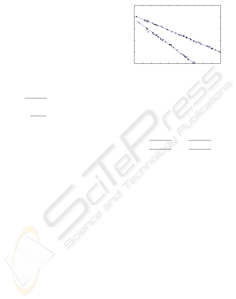
Figure 1: An example data set and corresponding (true) pair
of lines.
where D
c
= diag(λ
1
,λ
2
, 0). The corrected estimate
C
c
now perfectly satisfies the singularity constraint.
This estimate can further be reinterpreted in accor-
dance with the geometric nature of the associated set
Z
C
c
.Ifλ
1
and λ
2
are of opposite signs, then Z
C
c
is
the pair of lines
l
1
=
sgn(λ
1
)λ
1
v
1
+
sgn(λ
2
)λ
2
v
2
,
l
2
=
sgn(λ
1
)λ
1
v
1
−
sgn(λ
2
)λ
2
v
2
.
(7)
If λ
2
=0, then Z
C
c
is the double line v
1
.Ifλ
1
and
λ
2
are of same sign, then Z
C
c
represents the point
v
3
=[v
13
,v
23
,v
33
]
T
in P
2
, which, when v
33
=0,
belongs to R
2
and is given by [v
13
/v
33
,v
23
/v
33
, 1]
T
.
The last case can be viewed as exceptional and is not
expected to arise frequently. In a typical situation, the
input estimate C is such that the associated values λ
1
and λ
2
have opposite signs and the corrected estimate
C
c
is geometrically represented by the lines l
1
and l
2
given in (7).
7 EXPERIMENTS
To assess potential benefits stemming from the use
of constrained optimisation in the realm of GPCA,
we carried out a simulation study. Three algorithms,
ALS, HEIV and PHC (described in Sections 4 and 5),
were set to compute a pair of lines from synthetic
data. We utilised a particular version of HEIV, namely
the reduced HEIV scheme, or HEIV without intercept,
that operates essentially over a subspace of the para-
meter space of one dimension less (Chojnacki et al.,
2004a). The covariances of the data employed by
HEIV and PHC were assumed to be the default 2 ×2
identity matrix corresponding to isotropic homoge-
neous noise in image measurement.
To create data for our study, we randomly gen-
erated 100 pairs of lines. Along each line, in a
VISAPP 2006 - IMAGE ANALYSIS
210

Table 1: Averages of testing results.
σ Method J
AML
Rank-2 J
AML
ALS 1.286 ×10
−1
2.060 × 10
1
0.1 HEIV 1.084 × 10
−2
8.421 × 10
−2
PHC 1.065 × 10
−2
1.065 × 10
−2
ALS 1.444 ×10
1
5.977 × 10
5
0.55 HEIV 4.098 1.801 × 10
2
PHC 9.190 9.195
ALS 2.779 ×10
2
5.448 × 10
2
1.0 HEIV 4.448 3.652 × 10
1
PHC 2.816 2.816
Table 2: Medians of testing results.
σ Method J
AML
Rank-2 J
AML
ALS 1.135 ×10
−2
1.113 × 10
−2
0.1 HEIV 9.517 × 10
−3
1.037 × 10
−2
PHC 9.713 × 10
−3
9.713 × 10
−3
ALS 3.738 ×10
−1
3.687 × 10
−1
0.55 HEIV 3.092 × 10
−1
3.277 × 10
−1
PHC 3.121 × 10
−1
3.121 × 10
−1
ALS 1.094 1.212
1.0 HEIV 9.498 × 10
−1
1.093
PHC 9.509 × 10
−1
9.509 × 10
−1
section spanning 100 pixels in the x direction, 100
points were generated by sampling from a uniform
distribution. To these points homogeneous zero-mean
Gaussian noise was added at three different levels
characterised by the standard deviation σ of 0.1, 0.55
and 1 pixel. This data was generated so as to repre-
sent the kinds of line segment that may be found by
an edge detector. An example of the data is given in
Figure 1.
Each estimator was applied to the points generated
from each of the 100 pairs of lines and the resulting
estimates were recorded and evaluated. As a measure
of performance, we used the AML cost function, with
the standard value of J
AML
averaged across the points
in the image.
To ensure that the outputs of the algorithms can
be interpreted as genuine pairs of lines, all estimates
were post-hoc EVD corrected. The J
AML
value of
the corrected estimates, Rank-2 J
AML
, is given in the
rightmost columns in Tables 1 and 2. It is this Rank-2
J
AML
number that is the most informative indicator
of the performance of a particular method.
Tables 1 and 2 give the cost function values for
3 types of estimates. Table 1 shows that, on aver-
age, HEIV is an effective minimiser of J
AML
, and
that PHC coupled with EVD correction produces bet-
ter results that the EVD-corrected HEIV scheme.
Moreover—and this is a critical observation—when
applied to the PHC estimate, EVD correction leaves
the J
AML
value virtually unaffected (unlike in the
case of the HEIV estimate, where EVD correction
markedly worsens the J
AML
value). This confirms
that the result of approximate constrained optimisa-
tion has an almost optimal form and that EVD correc-
tion in this case amounts to a tiny push, which can be
stably executed in the presence of noise.
Table 2 presents the results of the same tests but re-
ports the median, rather than mean, of the J
AML
val-
ues. As the median is usually more representative of
the central tendency of a sample set than the mean, Ta-
ble 2 provides a better indication of the performance
of the algorithms on a typical trial.
8 CONCLUSIONS AND FUTURE
WORK
We have presented a novel version of GPCA for the
case of fitting a pair of lines to data, with a message
extending to the general case of multi-component es-
timation. At the core of our formulation lies the re-
duction of the underlying estimation problem to min-
imisation of an error function having solid statistical
foundations, subject to a parameter constraint. We
have proposed a technique for isolating an approxi-
mate constrained minimiser of that function. Prelim-
inary experiments show that our algorithm provides
better results than the standard GPCA based on un-
constrained minimisation of the error function.
There are clearly a number of ways in which the
work reported in this paper can be extended. The case
of multiple lines can be approached starting from the
observation that equation (1) characterising a pair of
lines can equivalently be written as (l
1
⊗
s
l
2
)
T
(m ⊗
m)=0, where l
1
⊗
s
l
2
=(l
1
⊗ l
2
+ l
2
⊗ l
1
)/2
is the symmetric tensor product of l
1
and l
2
, and
⊗ denotes the Kronecker (or tensor) product. More
generally, the equation for an aggregate of k lines
is (l
1
⊗
s
··· ⊗
s
l
k
)
T
(m ⊗ ··· ⊗ m)=0, where
l
1
⊗
s
···⊗
s
l
k
=(k!)
−1
σ∈S
k
l
σ(1)
⊗···⊗l
σ(k)
and
S
k
is the symmetric group on k elements. It is known
that the totally decomposable symmetric tensors of
the form l
1
⊗
s
···⊗
s
l
k
constitute an algebraic va-
riety within the space of all symmetric tensors (Lim,
1992). However, no explicit formula for the under-
lying constraints is known (this is a fundamental dif-
ference with the case of totally decomposable anti-
symmetric tensors). Working out these constraints in
concrete cases like those involving low values of k
will immediately allow the new version of GPCA to
cope with larger multi-line structures. More gener-
CONSTRAINED GENERALISED PRINCIPAL COMPONENT ANALYSIS
211

ally, progress in applying the constrained GPCA to
estimating more complicated multi-component struc-
tures will strongly depend on successful identification
of relevant constraints.
REFERENCES
(2003). Proc. IEEE Conf. Computer Vision and Pattern
Recognition.
Brooks, M. J., Chojnacki, W., Gawley, D., and van den Hen-
gel, A. (2001). What value covariance information in
estimating vision parameters? In Proc. Eighth Int.
Conf. Computer Vision, volume 1, pages 302–308.
Chojnacki, W., Brooks, M. J., van den Hengel, A., and
Gawley, D. (2000). On the fitting of surfaces to data
with covariances. IEEE Trans. Pattern Anal. Mach.
Intell., 22(11):1294–1303.
Chojnacki, W., Brooks, M. J., van den Hengel, A., and
Gawley, D. (2004a). From FNS and HEIV: A link be-
tween two vision parameter estimation methods. IEEE
Trans. Pattern Anal. Mach. Intell., 26(2):264–268.
Chojnacki, W., Brooks, M. J., van den Hengel, A., and
Gawley, D. (2004b). A new constrained parameter es-
timator for computer vision applications. Image and
Vision Computing, 22:85–91.
Chojnacki, W., Brooks, M. J., van den Hengel, A., and
Gawley, D. (2005). FNS, CFNS and HEIV: A
unifying approach. J. Math. Imaging and Vision,
23(2):175–183.
Duda, R. O. and Hart, P. E. (1972). Use of the Hough trans-
form to detect lines and curves in pictures. Commun.
ACM, 15:11–15.
Fitzgibbon, A., Pilu, M., and Fisher, R. B. (1999). Direct
least square fitting of ellipses. IEEE Trans. Pattern
Anal. Mach. Intell., 21(5):476–480.
Forsyth, D. A. and Ponce, J. (2003). Computer Vision: A
Modern Approach. Prentice Hall.
Hal
´
ı
ˇ
r, R. and Flusser, J. (1998). Numerically stable direct
least squares fitting of ellipses. In Proc. Sixth Int.
Conf. in Central Europe on Computer Graphics and
Visualization, pages 125–132.
Ho, J., Yang, M.-H., Lim, J., Lee, K.-C., and Kriegman,
D. J. (2003). Clustering appearances of objects un-
der varying illumination conditions. In (CVP, 2003),
pages 11–18.
Horn, R. and Johnson, C. (1985). Matrix Analysis. Cam-
bridge University Press, Cambridge.
Kanatani, K. (1996). Statistical Optimization for Geometric
Computation: Theory and Practice. Elsevier, Amster-
dam.
Leedan, Y. and Meer, P. (2000). Heteroscedastic regression
in computer vision: Problems with bilinear constraint.
Int. J. Computer Vision, 37(2):127–150.
Leonardis, A., Bischof, H., and Maver, J. (2002). Multiple
eigenspaces. Pattern Recognition, 35(11):2613–2627.
Lim, M. H. (1992). Conditions on decomposable symmetric
tensors as an algebraic variety. Linear and Multilinear
Algebra, 32:249–252.
Lou, X.-M., Hassebrook, L. G., Lhamon, M. E., and Li,
J. (1997). Numerically efficient angle, width, offset,
and discontinuity determination of straight lines by
the discrete Fourier-bilinear transformation algorithm.
IEEE Trans. Image Processing, 6(10):1464–1467.
Matei, B. and Meer, P. (2000). A general method for errors-
in-variables problems in computer vision. In Proc.
IEEE Conf. Computer Vision and Pattern Recognition,
volume 2, pages 18–25.
Nievergelt, Y. (2004). Fitting conics of specific types to
data. Linear Algebra and Appl., 378:1–30.
O’Leary, P. and Zsombor-Murray, P. (2004). Direct and spe-
cific least-square fitting of hyperbolæ and ellipses. J.
Electronic Imaging, 13(3):492–503.
Tipping, M. E. and Bishop, C. M. (1999). Mixtures of prob-
abilistic principal component analysers. Neural Com-
putation, 11(2):443–482.
Venkateswar, V. and Chellappa, R. (1992). Extraction of
straight lines in aerial images.
IEEE Trans. Pattern
Anal. Mach. Intell., 14(11):1111–1114.
Vidal, R. and Ma, Y. (2004). A unified algebraic approach
to 2-D and 3-D motion segmentation. In Proc. Eighth
European Conf. Computer Vision, volume 3021 of
Lecture Notes on Computer Vision, pages 1–15.
Vidal, R., Ma, Y., and Piazzi, J. (2004). A new GPCA al-
gorithm for clustering subspaces by fitting, differenti-
ating and dividing polynomials. In Proc. IEEE Conf.
Computer Vision and Pattern Recognition, volume 1,
pages 510–517.
Vidal, R., Ma, Y., and Sastry, S. (2003). Generalized prin-
cipal component analysis (GPCA). In (CVP, 2003),
pages 621–628.
Vidal, R., Ma, Y., and Sastry, S. (2005). Generalized princi-
pal component analysis (GPCA). IEEE Trans. Pattern
Anal. Mach. Intell., 27(12):1945–1959.
Vidal, R., Ma, Y., Soatto, S., and Sastry, S. (2002).
Segmentation of dynamical scenes from the multi-
body fundamental matrix. In ECCV Workshop
“Vision and Modelling of Dynamical Scenes”.
Available at http://www.robots.ox.ac.uk/
∼
awf/eccv02/vamods02-rvidal.pdf.
Vidal, R., Ma, Y., Soatto, S., and Sastry, S. (2006). Two-
view multibody structure from motion. Int. J. Com-
puter Vision. In press.
VISAPP 2006 - IMAGE ANALYSIS
212
