
CONSIDERATIONS ON THE FFT VARIANTS FOR AN EFFICIENT
STREAM IMPLEMENTATION ON GPU
Jos
´
e G. Marichal-Hern
´
andez, Fernando Rosa and Jos
´
e M. Rodr
´
ıguez-Ramos
Universidad de La Laguna. Depto. F
´
ısica Fund. yExp., Electr
´
onica y Sistemas.
Avda. Francisco S
´
anchez s/n, 38200 La Laguna, Tenerife, Canary Islands, Spain.
Keywords:
FFT, Graphics processing units, Stream computing, Signal processing, Image processing.
Abstract:
In this article, the different variants of the fast Fourier transform algorithm are revisited and analysed in terms
of the cost of implementing them on graphics processing units. We describe the key factors in the selection of
an efficient algorithm that takes advantage of this hardware and, with the stream model language BrookGPU,
we implement efficient versions of unidimensional and bidimensional FFT. These implementations allow the
computation of unidimensional transform sequences of 262k complex numbers under 13 ms and bidimensional
transforms on sequences of size 1024x1024 under 59 ms on a G70 GPU, that is almost 3.4 times faster than
FFTW on a high-end CPU.
1 INTRODUCTION
The fast Fourier transform (FFT) is a computational
tool of capital importance in almost every field of
science and engineering, where the faster the FFT is
computed, the better. Several visualization algorithms
spend part of their time performing domain trans-
forms to operate on data in the domain with the least
computational complexity. It can be also interesting
to reduce computation time when managing large se-
quences of data to make the FFT applicable in time-
critical computational problems. Of course, the FFT
is a key issue in digital signal processing, and that in-
cludes image and volume processing.
Graphics processing units (hereafter, GPUs) have
appeared in the last four years and, because of their
computational capabilities and because their adver-
tised and measured performance is several times
greater than that of high-end CPUs, have quickly
evolved to become considered as a generic computa-
tion platform, thereby taking them beyond their orig-
inal exclusively graphical purposes. A developer’s
meeting point where the history and evolution of the
GPU applied to generic computations can be found in
the GPGPU forum (GPG, na).
This article briefly reviews the implementations of
the FFT on GPUs to date and describes FFT variants
in an intuitive way that allows a choice to be made
of the most apropriate one to the stream processing
model. We analyse stream manipulation performance
to achieve an efficient mapping of the chosen FFT and
then we give implementation details of 1D and 2D
FFTs on a stream language for GPUs. Finally, the
performance of our implementation is analysed and
the future work is outlined.
2 RELATED WORKS
Several works have appeared over the last two years
proposing FFT implementations on GPUs the first of
these by Moreland and Angel (Moreland and Angel,
2003). Despite the proven computational power of
GPUs, this implementation did not succeed beating
the performance of the de facto standard implementa-
tion of the FFT on the PC platform, FFTW (Frigo and
Johnson, 2005).
Successive implementations (Wloka, 2003), (Viola
et al., 2004) have improved the performance of More-
land’s, but even in the best cases they were merely
equivalent to FFTW and, as well as Moreland and An-
gel did, they choose to implement the original FFT
variant from Cooley & Tukey (Cooley and Tukey,
1965).
The implementation proposed by Schiwietz and
Westermann (Schiwietz and Westermann, 2004) im-
proves the performance by formulating the discrete
Fourier transform, DFT, problem as a matrix multipli-
80
G. Marichal-Hernández J., Rosa F. and M. Rodríguez-Ramos J. (2006).
CONSIDERATIONS ON THE FFT VARIANTS FOR AN EFFICIENT STREAM IMPLEMENTATION ON GPU.
In Proceedings of the First International Conference on Computer Vision Theory and Applications, pages 80-86
DOI: 10.5220/0001361900800086
Copyright
c
SciTePress
cation, and the FFT as a process for decomposing and
factorizing the matrix in order to obtain sparse matri-
ces. Detailed explanations of this approach are to be
found in (Nussbaumer, 1982). An alternative unifying
theory of FFT variants is based on tensor products,
as is well documented in (Loan, 1992). These nota-
tions are especially powerful in performing automatic
search engines of the best algorithm for a specific ma-
chine, as in SPIRAL(P
¨
uschel and et al., 2005). An-
other way of expressing FFT variants consists in de-
composing the indices that appear in the DFT sum-
mations and reducing the number of operations on the
basis of discrete complex exponential properties and
a divide and conquer approach. An overview on this
technique can be found in (Swarztrauber, 1987).
The most efficient implementation (for GPUs) to
date is due to Jansen et al. (Jansen et al., 2004), whose
gain in performance relies on the named Split-stream-
FFT, although the algorithm is equivalent to that orig-
inally developed by Pease (Pease, 1968).
3 THE DFT AND FFT VARIANTS
The discrete Fourier transform of a 1D complex se-
quence, x(n), of size N is computed as
X(k)=
N−1
n=0
x(n) · W
kn
N
, 0 ≤ k<N (1)
W
nk
N
= e
−i2π
kn
N
If N =2
r
then indices n and k can be expressed in
binary using the index function I:
n =I(n
r−1
,n
r−2
,...,n
1
,n
0
)=
2
r−1
n
r−1
+2
r−2
n
r−2
+ ···+2n
1
+ n
0
; (2a)
k =I(k
r−1
,k
r−2
,...,k
1
,k
0
)=
2
r−1
k
r−1
+2
r−2
k
r−2
+ ···+2k
1
+ k
0
(2b)
Substituting these indices into eq. 1 gives
X(k
r−1
,...,k
0
)=
1
n
r−1
=0
...
1
n
0
=0
x(n
r−1
,...,n
0
)
· W
(2
r−1
k
r−1
+···+k
0
)(2
r−1
n
r−1
+···+n
0
)
2
r
(3)
Note that discrete complex exponentials verify that
W
zN
N
≡ 1, for z ∈ Z, and that, thus, every combi-
nation (k
i
,n
j
) with i + j ≥ r is cancelled out. The
process of reducing operations will be described for a
problem involving a size N =8,r=3:
1
n
2
=0
1
n
1
=0
1
n
0
=0
x(n
2
,n
1
,n
0
)
· W
(2
2
k
2
+2
1
k
1
+2
0
k
0
)(4n
2
+2n
1
+n
0
)
8
,
1
n
0
=0
1
n
1
=0
1
n
2
=0
x(n
2
,n
1
,n
0
)
·W
4k
2
(
4n
2
+
2n
1
+n
0
)+2k
1
(
4n
2
+2n
1
+n
0
)+k
0
(4n
2
+2n
1
+n
0
)
8
,
1
n
0
=0
1
n
1
=0
1
n
2
=0
x(n
2
,n
1
,n
0
)
· W
k
0
(4n
2
+2n
1
+n
0
)
8
· W
k
1
(2n
1
+n
0
)
4
· W
k
2
n
0
2
In this way, the most inner summation, with index n
2
,
can be collapsed and gives rise to a new arrangement
of the data sequence, X
1)
, expressed in terms of the
remaining indices in the time domain, n
0
and n
1
, and
the new frequency index k
0
:
1
n
0
=0
1
n
1
=0
X
1)
(k
0
,n
1
,n
0
)
1
n
2
=0
x(n
2
,n
1
,n
0
) · W
k
0
(4n
2
+2n
1
+n
0
)
8
· W
k
1
(2n
1
+n
0
)
4
· W
k
2
n
0
2
To accomplish the computation of X(k) this opera-
tion is repeated r times. At stage l, “index substitu-
tion”
n
r−l
+3
k
l
is performed:
1
n
0
=0
X
2)
(k
0
,k
1
,n
0
)
1
n
1
=0
X
1)
(k
0
,n
1
,n
0
) · W
k
1
(2n
1
+n
0
)
4
·W
k
2
n
0
2
,
1
n
0
=0
X
2)
(k
0
,k
1
,n
0
) · W
k
2
n
0
2
X
3)
(k
0
,k
1
,k
2
)
In fact, what has been done is a reformulation of the
problem as a multidimensional transform, each binary
dimension being transformed at a different stage. The
obtained sequence X
3)
is the bit-reversed index dis-
crete transform of the input sequence:
X(k)=X(k
2
,k
1
,k
0
)=
= bitReversedIndex(X
3)
(k
0
,k
1
,k
2
))
The algorithm described corresponds to that pro-
posed by Cooley and Tukey for a size N =2
r
(radix-
2). The final bit reversal on the indices on the trans-
formed domain is also called decimation-in-frequency
(DIF).
The order of the index substitution is fixed:
n
r−1
+3
k
0
, ...,
n
0
+3
k
r−1
. But playing
CONSIDERATIONS ON THE FFT VARIANTS FOR AN EFFICIENT STREAM IMPLEMENTATION ON GPU
81

with the positions in sequence X
l−1)
, where n
r−l
“disappears”, and the position in X
l)
, where k
l
“ap-
pears”, creates variants of the FFT. Figure 1 shows
in an intuitive way the FFT variants due to Stock-
ham (Stockham, 1966) and Pease (Pease, 1968), as
well as DIT and DIF versions of C&T (Cooley and
Tukey, 1965) for a size 8 sequence.
a)
n
2
n
1
n
0
k
0
n
1
n
0
k
0
k
1
n
0
k
0
((
R
R
R
R
R
R
k
1
k
2
vv
m
m
m
m
m
m
k
2
k
1
k
0
b)
n
2
))
S
S
S
S
S
S
n
1
n
0
uu
k
k
k
k
k
k
n
0
n
1
n
2
n
0
n
1
k
0
n
0
k
1
k
0
k
2
k
1
k
0
c)
n
2
n
1
n
0
k
0
n
1
y
z
z
z
z
n
0
k
1
k
0
n
0
rz
m
m
m
m
m
m
m
m
m
m
m
m
k
2
k
1
k
0
d)
n
2
))
S
S
S
S
S
S
n
1
n
0
uu
k
k
k
k
k
k
n
0
n
1
n
2
qy
l
l
l
l
l
l
l
l
l
l
l
l
k
0
n
0
n
1
rz
m
m
m
m
m
m
m
m
m
m
m
m
k
1
k
0
n
0
rz
m
m
m
m
m
m
m
m
m
m
m
m
k
2
k
1
k
0
Figure 1: FFT variants. From left to right, and top to bot-
tom: a) Cooley & Tukey radix-2 decimation-in-frequency,
and b) decimation-in-time. Cooley and Tukey variants per-
forms in-place index substitution with bit-reversed input
and ordered output if DIF. c) shows the Stockham variant.
The index substitution is out of place, but no scramble on
the data is necessary. d) corresponds to Pease. Index sub-
stitution is the same at every stage: time indices disappear
from the least significant position and their frequency coun-
terparts appear at the most significant one.
We now consider the computational consequences
of following one or other of these schemes. Two el-
ements from X
l−1)
are needed to compute one ele-
ment of X
l)
. In fact, two output elements can be
computed with the same two input elements. This
is called a butterfly operation, and relates a pair of
dual nodes between a stage and the following. The
distance in memory, stride, between the two input el-
ements involved in the butterfly is given by the sig-
nificance of the binary index that disappears. The
stride of the computed elements in the resulting se-
quence is given by the significance with which the
new frequency index appears. For example, substitu-
tion
n
2
+3
k
0
in the C&T DIF scheme, in which
both indices appear in and disappear from the most
significant index position can be thought as retriev-
ing pairs of data with distance N/2 (the weight of
the index position in the index function I), combin-
ing them with the appropriate discrete complex ex-
ponential and leaving new data in the same sequence
positions, therefore equally distanced N/2. Never-
theless, a substitution like those in the Pease variant,
where indices disappear from the least significant po-
sition and appear in the most significant one, implies
retrieving data with unitary stride but depositing them
with maximum stride. The Stockham variant distrib-
utes the decimation step among the stages.
Only in the Pease variant are the input and output
strides independent of the stage being performed. The
out-of-place condition of Pease and Stockham vari-
ants can be partly avoided by performing an in-place
computation and then a suitable output recombina-
tion.
4 COMPUTATIONAL
FRAMEWORK
Because GPUs were usually found in the context of
computer graphics, the programming languages and
techniques involved have been inherently graphics-
related. Knowledge of graphics APIs such as
OpenGL and fragment programming languages such
as Cg were needed. In order to get maximum per-
formance, an extensive knowledge of state-of-the-art
extensions was also required.
BrookGPU (Buck et al., 2004) is a subset of the
brook language (Buck, 2004) developed in the Mer-
rimac processor (Dally et al., 2003) project. One
big contribution of a language like BrookGPU is
to propose an abstract computing model, the stream
processing model, that can effectively retain and em-
phasize GPU main characteristics but at a more con-
ceptual level than used to be the case. In this way,
not only is GPU programming detached from graph-
ics concerns but also developers can concentrate on
choosing a meaningful stream algorithm yielding the
gap from generality to efficiency to BrookGPU devel-
opers.
The main capabilities of GPUs are inherited by
BrookGPU streams, the data structures in BrookGPU,
and by kernels, the programs that operate on them.
BrookGPU’s maximum performance is achieved
when an algorithm takes full advantage of the GPU
resources. In this sense, the GPU’s computational
power is based on its ability to operate in four com-
ponent registers, each with 32 bit floating point pre-
cision. The GPU instruction set operates in a 4-wide
SIMD parallel manner, and it is oriented to perform
4-vector and 4×4-matrix operations. Nevertheless,
bit operations are not available. On the older GPUs,
dynamic branching is forbidden and one kernel is re-
stricted to giving one stream as output, whereas newer
GPUs are able to contain loops and to output up to
four streams at the same time. We will make no use
of these advanced features in our implementation.
VISAPP 2006 - IMAGE FORMATION AND PROCESSING
82

Kernels generate each element of the output stream
combining the element from each input stream that
maps on the position being computed. That is, when
generating the stream element (strel from now on,
for simplicity) that occupies position i at the out-
put stream, the kernel operates exclusively with input
strels at position i.
Kernel inputs, as well as streams, can be constants
and gatherable streams. Gatherable streams violate
the preceding statement and allow strels to be fetched
from any position. Nevertheless, their use is not rec-
ommended because they rely upon texture fetches.
These accesses are not necessarily slower than di-
rect stream mapping, but the direct stream mapping
approach explicitily strenghtens cache coherency. A
special type of kernel that equally violates the preced-
ing statement are known as reductions. In reduction
kernels output streams have fewer elements than in-
put streams so they combine several strels from each
input stream. They are conceptually powerful, but
their use is also inadvisable because their poor per-
formance.
Streams can be 1D and 2D, and soon 3D, and
the strels can hold 1 to 4 floats. A typical max-
imum allowable size for a 2D stream nowadays is
4096 × 4096.
Some rules applied by BrookGPU to fit streams of
different sizes participating in a kernel are essential
for understanding the mapping between input and out-
put strels. These are:
• The dimensionality in which a kernel operates is
that of the output stream. Input streams must have
the same number of dimensions as the kernel.
• The size of a kernel is that of its output stream.
• For every input stream, and for every dimension in-
dividually, the following rules are applied to fit in-
put stream sizes to kernel size:
– if the stream size is bigger than the kernel size by
an integer factor N, just 1 from every N strels
participates in the kernel. This is called implicit
striding; e.g. stride
(N=2)
{abcd}→{ac}
– if the kernel size is bigger than the stream size
by an integer factor N , each strel is repeated
N times. This is called implicit repetition; e.g.
repeat
(N=2)
{abcd}→{aabbccdd}
Before applying the above rules, the streams par-
ticipating in a kernel can be passed through a domain
operator. This operator allows the selection of a re-
gion of the whole stream, indicating a beginning and
an end; e.g. domain
(start=2,end=3)
{abcd}→{cd}.
The domain operator modifies the way that the af-
fected stream maps on to a kernel without additional
cost. Moreover, its use in output streams allows ker-
nel sizes to be decreased.
Figure 2: FFT on multiple 1D sequences of data arranged
across rows of a 2D stream. a) Distance in a row of the
stream for least and most significat bits. b) Complex butter-
fly operation performed on a 4-wide SIMD within 1 stream
element. c) Redistribution of elements in a row of the
stream: lsb neighbours A, B finish at distance MSB. C and
D, which started in an odd column, finish in second slot of
a strel. d) Pease FFT in terms of streams and kernels. ec
and oc stand for the domain operators that select just even
or odd columns. Similarly, fhh and shh stand for first and
second horizontal half.
The domain operator can be thought of as the ex-
plicit user side counterpart of the stride and repeats
implicit rules. By making suitable use of both, a
somewhat more complicated mapping pattern can be
achieved. For example,
foo ( domain
start=(1,0),end=(N +1,M )
{inX},
domain
s=(0,0),e=(N/2,M)
{outY } )
maps the odd rows of a 2D input stream inX of size
N×M , on to the first vertical half of the output stream
outY.
5 EFFICIENT STREAM
IMPLEMENTATION
In order to obtain an efficient stream implementa-
tion of the FFT, an adequate variant must be chosen
that takes into account the advantages of GPUs, while
avoiding those aspects that are known to give a poor
performance. This implies making an effort to move
and operate data in a 4-wide manner, which in terms
of BrookGPU means operating on float4 streams, em-
ploying domain and implicit size reaccommodation
whenever they can replace the expensive gatherable
streams, avoiding the reductions, yielding to CPU
those computations that are impossible or too hard to
carry out on the GPU, and making kernel executions
as regular as possible.
The FFT variants in Fig. 1 can be now analysed in
terms of stream costs. The data strides in the Stock-
ham and C&T variants depend on the stage being
performed. To implement these strides exclusively
as a stream mapping is impossible or much too ex-
pensive. An alternative is to make use of gatherable
CONSIDERATIONS ON THE FFT VARIANTS FOR AN EFFICIENT STREAM IMPLEMENTATION ON GPU
83

streams and dependent fetches. In contrast to this
approach, the Pease variant has a remarkable prop-
erty; the butterfly input strides are unitary and stage-
independent. This allows us to perform the butterfly
operation within a strel, beacuse two complex num-
bers can be stored within a float4 strel. To compute
butterfly on them only the appropriate complex expo-
nential is needed, and no other element in data stream
is involved. Hence, if the results are stored in-place,
direct mapping can be applied from the input to the
output stream. This takes full advantage of the GPU
memory bandwidth. The disadvantage is that a re-
combination step must be performed after butterfly
computations. See the Fig. 2.a and Fig. 2.b.
Butterfly computation, once appropriate data are
available in a kernel, is trivial and can be efficiently
performed in a 4-wide SIMD manner.
Determining complex exponentials W
nk(l)
N(l)
in-
volves not only operating with trigonometric func-
tions but also performing stage-dependent bit level
manipulations on the strel positions. A better perfor-
mance is obtained precomputing these values in CPU.
Another technique that should be analysed in terms
of stream costs is the index bit reversal. Explaining it
in actual BrookGPU code exemplifies several of the
previously described ideas about stream operations.
In this example, it is assumed that one strel holds two
complex data that in the original sequence are least
significant bit, lsb, adjacents.
First, split a sequence of size N on 2 sequences of
size N/2, which differ only in the most significant bit,
MSB. Both N/2 sequences can be index bit reversed
separately using the same bit-reversal pattern. In or-
der to obtain the bit reversed complete sequence, both
half sequences must then be merged with unit stride:
0123 4567 →
0
0
123|
4
0
123 →
0
0
213|
4
0
213 → 04 26 15 37
The idea consists in performing MSB ↔ lsb inter-
change separately, based more upon stream opera-
tions than that of the rest of the bits, based on a pre-
calculated interchange pattern.
In the following code, the 2D stream of float2 ele-
ments X is bit reversed and packed into float4 stream
Xr with half of the elements in horizontal. The stream
br holds the bit-reversal pattern. Note the mechanism
to load data to the streams, and the way BrookGPU
sentences are inserted into C code:
float2 X<N,M>, br<N, M/2>;
float4 Xr<N, M/2>;
float2 data_br[N][M/2], data_X[N][M];
for (i=0; i < N; i++)
for (j=0; j < M/2; j++) {
br[i][j].x = bitReverse(j);
br[i][j].y = bitReverse(i);
}
dataRead(br, data_br);
dataRead(X, data_X);
The kernel declaration that performs the bit-
reversal and the packing of the two sequences is very
simple. The first two inputs to the kernel are gather-
able streams. The appropriate position from which
those inputs must be fetched were precomputed and
passed through the third input, a (non-gatherable)
stream. The kernel code itself just forwards com-
plex numbers fetched from first and second half of
the original stream to the appropriate slot (.xy or .zw)
in the output strel:
kernel void reverseKernel(float2 X_0_M2[][],
float2 X_M2_M[][],
float2 br<>,
out float4 result<>) {
result.xy = X_0_M2[br];
result.zw = X_M2_M[br];
}
The domain operators, applied in the kernel call, split
horizontally the X stream:
reverseKernel(X.domain(int2(0,0), int2(M/2,N)),
X.domain(int2(M/2,0), int2(M,N)),
br, Xr);
The gain obtained by the unitary input stride of
the Pease algorithm has its counterpart in an addi-
tional recombination step to leave lsb adjacent data in
the MSB stride (see Fig. 2.c). However, that recom-
bination can be accomplished using the same tech-
niques explained above for bit-reversal. The splitting
is achieved by a suitable use of the domain operator,
and the merging is done via a data-forwarding kernel.
The Pease variant therefore has several advantages
over other FFT variants, and its disadvantages can be
partially overcome using domain operations and data-
forwarding kernels.
5.1 The FFT of Multiple Regular
Sized 1D Sequences
Implementing small (less than 1 × 2048) FFTs on
GPUs has limited benefits. GPU FFTs are more valu-
able when faced with bigger problems.
The techniques previously outlined in this section
when applied to a stream of size 1 × M perform a
1D FFT, but when applied to a stream of size N × M
solves in parallel N 1D FFTs of size M .
Figure 2.d shows the relationship between the
streams and kernels that perform one of the log
2
(M)
required stages. The X stream has size N ×M/2 after
the complex input data have been index bit reversed
and packed into float4 elements.
When X is split horizontally into X
ec
and X
oc
, the
resulting streams are of size N × M/4. Having two
butterfly kernels allows to store two complex expo-
nentials in each element of the W stream. The code in
both kernels differs only in the W slot being used (.xy
for even columns). The W stream has size 1 × M/4.
The replication along the N rows is free.
After X
ec
and X
oc
are computed, they must be re-
combined. From the Fig. 2.c, it can be seen that each
strel in the first horizontal half of Y gets its first slot
from the first slot in X
ec
and the second slot from the
VISAPP 2006 - IMAGE FORMATION AND PROCESSING
84
first slot in X
oc
. This is done by kernel combineXY().
Kernel combineZW() combines the second slots from
X
ec
and X
oc
in the second horizontal half of Y .
Stream W is stage-dependent. However, the W
stream in one stage is composed of a half of the val-
ues in the previous stage. Only the initial W must
be computed in CPU, while the following ones can
be efficiently updated in GPU via a modulus opera-
tion. The decreasing diversity of W values allows us
to make use of simplified butterfly kernels in the last
two stages.
5.2 2D FFT as 2 Consecutive 1D FFT
An FFT on a 2D sequence of size N × M can be per-
formed by consecutively applying N 1D transforms
along the rows and then M 1D transforms along the
columns.
To apply exactly the same stream approach as in
previous subsection, two additional transpositions of
data are necessary, the first being applied after com-
puting the N 1D FFT’s of size M along the rows.
The transposition reshapes the data sequence into an
M × N stream with data already transformed along
the columns. Again, the same multiple 1D FFTs can
be performed along rows, simply changing the size
of transforms, now N. These size differences only
imply subtle changes to stream W , which now must
be of size 1 × max(N,M ). A final transposition is
required to recover the original shape.
The algorithm could be reformulated to perform di-
rectly along columns, but in that case lsb adjacency
falls outside the strel boundaries and the performance
drops.
The difficulty in transposing the stream is that
along horizontal dimension one the strel holds two
complex data, while on the other the relation is 1:
1. If both relations were the same, the transposi-
tion would be completed with a dependent reading
of the original data with the indices of the current
kernel position interchanged (xy → yx): X
T
=
X[indexOf(X
T
).yx]
To take this asymmetry into account, the old x in-
dex must be multiplied and y index divided by 2. As
long as one output must contain two complex data
placed in consecutive columns, two fetches, from 2x
and 2x +1, are required. This renders 4 complex
numbers, two of which are discarded depending on
the remainder y/2.
5.3 FFT of Large 1D Sequences
A 1D sequence can be arranged in a 2D stream by
storing it in a row-wise manner. In this way, a se-
quence of 262k elements can fit into a 512 × 512 2D
stream. The Pease algorithm is still applicable, but
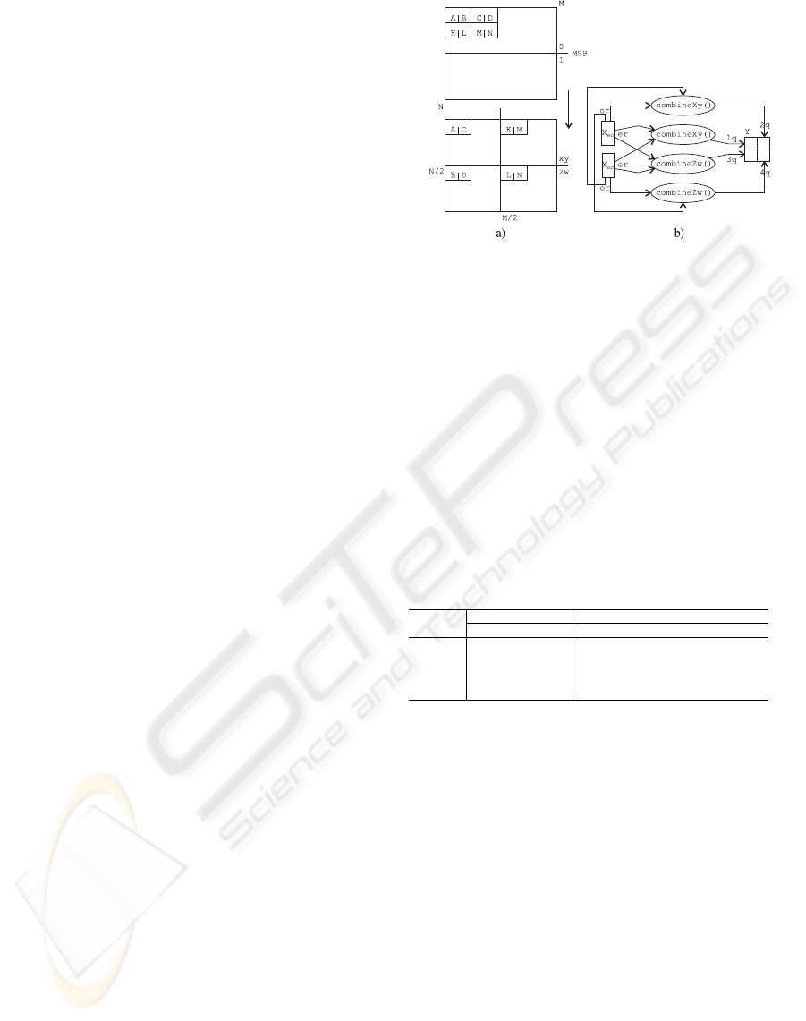
Figure 3: The FFT on a 1D sequence of data arranged across
a 2D stream in row-wise order. a) The MSB divides the
data vertically. The elements starting from positions with
lsb =0, such as A, C, K and M, fall on first vertical half
of the stream. The elements starting in even rows, such as
A, B, C and D, fall in the first horizontal half of the stream.
These two combinations give up the four quarters of the
output stream. b) Kernels and streams involved in the re-
combination step. The results from butterfly kernels, stored
in Xec and Xoc streams, are recombined into the four quar-
ters of the output allowing for the possibilities lsb=0/1 and
even/odd rows.
Table 1: Times to perform an FFT on sequences of complex
numbers, with a G70 GPU. The first two columns contain
the times to transfer data to and from the GPU. The second
block of columns contains the computation times for: N 1D
FFTs of size N, 1D FFTs of size N
2
and 2D FFTs of size
N × N .
Problem Transfer times (ms) Computation time (ms)
size: N C→ GG→ C N 1D N 1D N
2
2D N × N
64 0.03 0.09 0.85 1.89 1.74
128
0.21 0.22 1.18 2.34 2.27
256
1.16 0.7 1.9 3.1 3.8
512
4.6 3.0 6.6 12.8 13.7
1024
18.3 12.3 27 56 58
the new arrangement of data must be taken into ac-
count when precomputing W and on the recombina-
tion steps.
Figure 3.a shows the implications for lsb and MSB
adjacency from such an arrangement, and the Fig. 3.b
contains the stream operations to perform the proper
recombination.
The number of different values of the W stream
halves at each stage, but the modulus operation across
the two dimensions requires more time than bind-
ing a suitable one from an array of precomputed
streams,W[l].
6 PERFORMANCE AND
CONCLUSION
The following results were obtained using BrookGPU
(brcc version 0.2, March 2005), with the OpenGL
CONSIDERATIONS ON THE FFT VARIANTS FOR AN EFFICIENT STREAM IMPLEMENTATION ON GPU
85

runtime, on a Windows XP platform (Linux version of
BrookGPU has an approx. 20% worse performance).
The graphics board used was a GeForce 7800 GTX
(G70 engine) connected to the host machine through
a PCI-Express slot on a nForce4 chipset motherboard.
The driver version was 76.67 (updated in June 2005).
Table 1 shows the times required for computing the
FFT on the GPU for several problem sizes. Data up-
load and download times are isolated from compu-
tation times, and penalize GPU use as a coprocessor
to the CPU for computing FFT. But for some appli-
cations, like medical imaging on precaptured data or
direct video manipulation on GPU, they are not re-
quired.
Computation times include the time consumed by
stream copies between kernels, but those times cannot
be broken down. The performance obtained is simi-
larly independent of the organization of the data. The
time to perform 1D FFT of size N
2
, doubles that of
performing N 1D FFTs of size N because twice the
stages must be performed. The difference between 1D
N
2
and 2D N × N is due to the transpositions.
These times, for the problems of bigger sizes are
3.4 times faster (58 vs 196 ms for 1024x1024 complex
size) than the FFTW library run on an AMD 3500+
CPU with 512KB of L1 cache.
6.1 Conclusion
Our implementation has a remarkable performance
and within the range of the fastest implementation
on GPU. Additionally a comprehensive framework in
which FFT variants and the stream model meet has
been discussed. The proposal and development of
new implementations can now be undertaken along
the lines suggested in this document.
For the future, we shall implement 2D transforms
that collapse the indices in two dimensions at a time.
We think these methods could be especially valuable
when working on GPUs that allow multiple outputs
per kernel.
ACKNOWLEDGEMENTS
This work has been partially supported by “Programa
Nacional de Dise
˜
no y Producci
´
on Industrial” (Project
DPI 2003-09726) of the “Ministerio de Ciencia y Tec-
nolog
´
ıa” of the spanish government, and by “Euro-
pean Regional Development Fund” (ERDF).
Jos
´
e G. Marichal-Hern
´
andez has awarded a grant
by “Becas de investigaci
´
on para doctorandos. Conve-
nio ULL–CajaCanarias 2005”.
The authors would like to thank Terry Mahoney for
a critical reading of the original version of the paper.
REFERENCES
(n.a.). General purpose computation using graphics hard-
ware. Developer’s forum. http://www.gpgpu.com/.
Buck, I. (2004). Brook specification v.0.2. Tech. Rep.
CSTR 2003-04 10/31/03 12/5/03, Stanford University.
Buck, I., Foley, T., Horn, D., Sugerman, J., Fatahalian, K.,
Houston, M., and Hanrahan, P. (2004). Brook for
GPUs: stream computing on graphics hardware. ACM
Trans. Graph., 23(3):777–786.
Cooley, J. W. and Tukey, J. W. (1965). An algorithm for the
machine calculation of complex fourier series. Math-
ematics of Computation, 19:297–301.
Dally, W. J., Hanrahan, P., Erez, M., Knight, T. J., and alter
(2003). Merrimac: Supercomputing with streams. In
SC’03, Phoenix, Arizona.
Frigo, M. and Johnson, S. (2005). The design and im-
plementation of FFTW3. In Proc. of the IEEE, vol-
ume 93, pages 216– 231. http://www.fftw.org.
Jansen, T., von Rymon-Lipinski, B., Hanssen, N., and
Keeve, E. (2004). Fourier volume rendering on the
GPU using a Split-Stream-FFT. In Proc. of the
VMV’04, pages 395–403. IOS Press BV.
Loan, C. V. (1992). Computational frameworks for the fast
Fourier transform. Society for Industrial and Applied
Mathematics, Philadelphia, PA, USA.
Moreland, K. and Angel, E. (2003). The FFT on a GPU. In
Proc. of the ACM SIGGRAPH, pages 112–119. Euro-
graphics Association.
Nussbaumer, H. J. (1982). Fast Fourier Transform and Con-
volution Algorithms. Springer-Verlag, second edition.
Pease, M. C. (1968). An adaptation of the fast fourier trans-
form for parallel processing. J. ACM, 15(2):252–264.
P
¨
uschel, M. and et al., J. M. F. M. (2005). SPIRAL: Code
generation for DSP transforms. Proc. of the IEEE,
93(2).
Schiwietz, T. and Westermann, R. (2004). GPU-PIV. In
Proc. of the VMV’04, pages 151–158. IOS Press BV.
Stockham, T. (1966). High speed convolution and correla-
tion. In AFIPS Proceedings, volume 28, pages 229–
233. Spring Joint Computer Conference.
Swarztrauber, P. N. (1987). Multiprocessor FFTs. Parallel
computing, 5(1–2):197–210.
Viola, I., Kanitsar, A., and Gr
¨
oller, M. E. (2004). Gpu-
based frequency domain volume rendering. In Proc.
of SCCG 2004, pages 49–58.
Wloka, M. M. (2003). Implementing a GPU-efficient FFT.
SIGGRAPH course slides.
VISAPP 2006 - IMAGE FORMATION AND PROCESSING
86
