
QUANTITATIVE COMPARISON OF TOLERANCE-BASED
FEATURE TRANSFORMS
Dennie Reniers, Alexandru Telea
Department of Mathematics and Computer Science, Eindhoven University of Technology
Den Dolech 2, 5600 MB, Eindhoven, The Netherlands
Keywords:
feature transform, tolerance-based, distance transform, algorithms, image processing.
Abstract:
Tolerance-based feature transforms (TFTs) assign to each pixel in an image not only the nearest feature pixels
on the boundary (origins), but all origins from the minimum distance up to a user-defined tolerance. In this
paper, we compare four simple-to-implement methods for computing TFTs on binary images. Of these meth-
ods, the Fast Marching TFT and Euclidean TFT are new. The other two extend existing distance transform
algorithms. We quantitatively and qualitatively compare all algorithms on speed and accuracy of both distance
and origin results. Our analysis is aimed at helping practitioners in the field to choose the right method for
given accuracy and performance constraints.
1 INTRODUCTION
A distance transform (DT) computes, for pixel p of an
image, the distance D(p) = min
q∈δΩ
kq − pk to the
nearest feature pixel, or origin, q on the boundary δΩ
of some object Ω located in the image. Non-object
pixels will be denoted by
¯
Ω. There can be several
equidistant origins q for a pixel p, i.e., the origin set
S(p) = arg min
q∈δΩ
kq −pk of p can have more than
one element. The feature transform (FT) assigns to
each pixel p the origin set S(p). A simple FT com-
putes only one origin per pixel, which is sufficient
for some applications. We define a tolerance-based
FT (TFT) as a map that assigns to each pixel the set
S
(p) = {q ∈ δΩ
kq −pk ≤ D(p)+ }, where is a
user-defined tolerance. One use of the TFT is to com-
pute exact Euclidean DTs, as first observed in (Mul-
likin, 1992) (see also Sec. 5). A second use of the TFT
is to compute robust, connected skeletons or medial
axes, as follows. Medial axis (MA) points can be de-
tected as the FT points having at least two origins, one
on each side of the axis (Foskey et al., 2003). How-
ever, this definition may yield disconnected skeletons
in a discrete space. For example, for a rectangle of
even width, no pixels lie exactly in the middle. Us-
ing a TFT with tolerance 1, origins from both axis
sides are found, yielding a connected skeleton. Over-
all, both DTs and FTs have numerous applications
in many domains (Cuisenaire, 1999; Ye, 2003) rang-
ing from image processing, pattern recognition, and
shape representation and modeling, to path planning,
computer animation, skeletonization, and optimiza-
tion algorithms.
DT and FT algorithms can be classified by the or-
der in which they process the image pixels. Raster
scanning algorithms (Danielsson, 1980) sequentially
process pixels in scan-line order, needing multiple
passes at which pixels are assigned new minimum
distances. Ordered propagation methods (Ragne-
malm, 1992) reduce the number of distance com-
putations needed by updating only pixels in a con-
tour set, which propagates from the object bound-
ary δΩ inwards. Ordered propagation methods ac-
commodate (distance-based) stopping criteria eas-
ier than raster scanning ones, thus being more effi-
cient for some applications. A well-known class of
ordered propagation methods are level-set and fast
marching methods (FMM) (Sethian, 1999), which
evolve the contour δΩ under normal speed (see
Section 2). Although the FMM does not com-
pute an exact Euclidean DT, the speed function it
uses can be locally varied to compute more com-
plex DTs, e.g., anisotropic, weighted, Manhattan, or
position-dependent ones (Sethian, 1999; Strzodka and
Telea, 2004). Recent FMM extensions compute an
FT (Telea and van Wijk, 2002; Telea and Vilanova,
2003). However, this is only a simple FT, and can
be quite inaccurate in many cases. Applications us-
107
Reniers D. and Telea A. (2006).
QUANTITATIVE COMPARISON OF TOLERANCE-BASED FEATURE TRANSFORMS.
In Proceedings of the First International Conference on Computer Vision Theory and Applications, pages 107-114
DOI: 10.5220/0001361801070114
Copyright
c
SciTePress

ing this origin set, such as skeletonization, can deliver
wrong results, as pointed out in (Strzodka and Telea,
2004).
As the above outlines, DT and FT methods have
many, often subtle, trade-offs, which are not obvious
to many practitioners in the field. In this paper, we
discuss several competitive DT, FT, and TFT meth-
ods. Some of these methods extend existing ones,
while others are new. We quantitatively and quali-
tatively compare the results of all methods with the
exact TFT computed by brute force, and discuss the
computational advantages and limitations of every
method. The goal of our analysis is to provide a quan-
titative, practical guideline for choosing the “right”
DT or (T)FT method to best match real-world appli-
cation requirements, such as precision, performance,
completeness, and implementation complexity.
This paper is structured as follows. In Section 2
we discuss the FMM and we detail on its inaccura-
cies. In Section 3, we modify the existing Augmented
Fast Marching Method (AFMM) to yield exact simple
FTs, and illustrate its use by skeletonization applica-
tions. In Section 4, we extend this idea to compute
TFTs by adding a distance-to-origin tolerance. In
Section 5, we analyze Mullikin’s raster scanning DT,
and get insight into how to set our TFT tolerance to
compute exact DTs. In Section 6, we present a novel
method, called ETFT, based on a different propaga-
tion order than the FMM. In Section 7, we compare
our new ETFT with the related graph-search method
of (Lotufo et al., 2000), and also extend the latter to
compute TFTs. Finally, we quantitatively compare all
of the above methods (Sec. 8) and come to a conclu-
sion (Sec. 9).
2 FAST MARCHING METHOD
(FMM)
Level set methods are an Eulerian approach for track-
ing contours evolving in time. The fast marching
method (FMM) (Sethian, 1999) treats the special case
of contours with constant sign speed functions F . The
contour position p, given by its arrival time T (p), is
the solution of k∇T kF = 1 with T = 0 for the initial
contour δΩ. If F = 1, we obtain the Eikonal equation
k∇T k = 1 whose solution is the Euclidean DT of δΩ.
The FMM efficiently computes T using the fact that
T (p) depends only on the T values of p’s neighbors
N(p) for which T (N (p)) < T (p). The FMM builds
T from the smallest computed T values by maintain-
ing the pixels in the evolving contour, or narrow band,
sorted on T . Pixels are split in three types: known pix-
els p
K
have an already computed T ; temporary pixels
(p
T
) have a T subject to update; and unknown pixels
(p
U
) have not yet been assigned a T value. Invariant
Table 1: Differences between (approximate) FMM and ex-
act Euclidean distances D (%e: ratio of erroneous pixels to
object pixels; max e: maximum error; ¯e: average error).
image img.size max D %e max e ¯e
bird 238×370 49.82 89% 0.679 0.142
leaf 410×444 70.63 84% 1.013 0.290
dent 464×397 134.06 15% 1.210 0.082
is T (p
K
) ≤ T (p
T
) ≤ T (p
U
). Initially, all pixels on δΩ
are known to have T = 0 and their neighbors become
temporary. Next, the temporary pixel p with smallest
T becomes known (as its T cannot be influenced by
other pixels), its unknown neighbors N
U
(p) become
temporary, and their T values are updated based on
their own known neighbors, until all pixels become
known. For a contour of length B = |δΩ| and area
N = |Ω| pixels, the FMM needs O(N log B) steps.
The DT computed by the FMM is not exact. Errors
occur due to the approximation of the gradient ∇T ,
usually of first or second order, the former being the
most common. The errors are accumulated during the
propagation. In (Sethian, 1999, Sec. 12.3), the FMM
accuracy is briefly treated, but no comments are made
on the implications for real-world applications. Fig-
ure 1 and Table 1 show the difference between the
FMM and the exact DT for some typical shapes. High
errors (bright areas in Fig. 1) seem to “diffuse” away
from boundary concavities. Indeed, a temporary point
at a narrow band concavity has just one known neigh-
bor N
K
, so its distance is updated from a single known
T (N
K
) value. A point at a narrow band convexity has
several known neighbors, so its distance T is updated
using more information. The maximal DT error can
easily exceed 1 pixel (cf. Table 1), and can grow arbi-
trarily with the image size.
3 AFMM STAR
In (Telea and van Wijk, 2002), the Augmented FMM
(AFMM) is presented, which computes one origin per
pixel by propagating an arc-length parameterization
U of the initial boundary δΩ together with FMM’s T
value. U(p) basically identifies an origin S(p). When
a narrow band pixel p is made known and its unknown
direct 4-neighbors a ∈ N
U
4
(p) are added to the nar-
row band, U (a) is set to U (p). After propagation
has completed, for all points q where U varies with
τ over N
4
(q), a segment of length τ from the orig-
inal boundary collapses. Hence, the above point set
{q} represents a (pruned) skeleton, or medial axis, of
δΩ. AFMM’s complexity remains the same as for the
FMM, namely O(N log B), where N is the number
of object pixels and B the boundary size, because it
VISAPP 2006 - IMAGE FORMATION AND PROCESSING
108
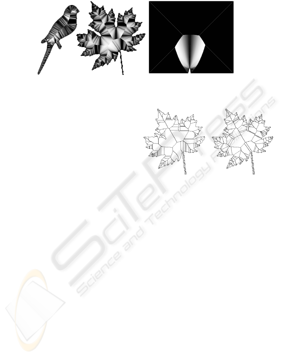
Figure 1: Differences between the (approximate) FMM distance and the exact Euclidean distance for the ‘bird’, ‘leaf’, and
‘dent’ images. Black indicates no error, white indicates the maximum error. See Table 1 for the exact values.
adds just the propagation of one extra value U. Sim-
ilar methods are (Costa and Cesar, 2001) for digital
images and (Ogniewicz and K
¨
ubler, 1995) for polyg-
onal contours, respectively.
However efficient and effective for computing sim-
ple FTs and skeletons, the AFMM has several ac-
curacy problems when computing U , as can be eas-
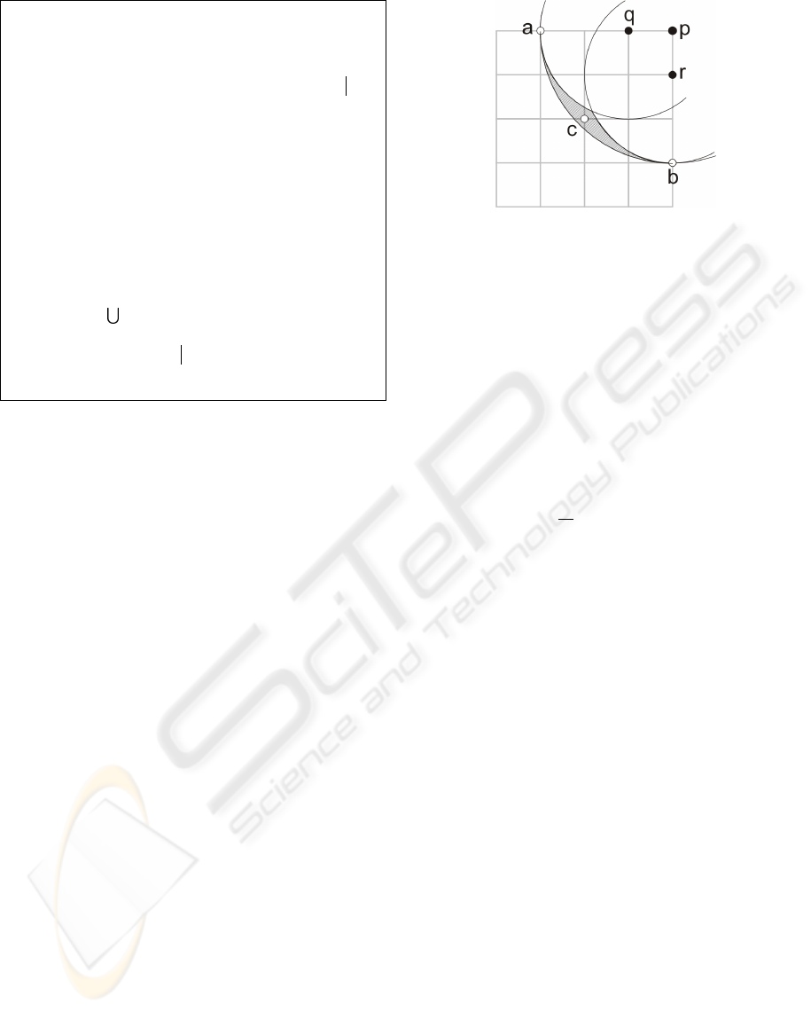
ily seen from the resulting skeletons. Errors show
up as skeleton branches having the wrong angle, are
too thick, or are disconnected (e.g., Fig. 2 left). The
reason is that the value U (a) is determined by only
one pixel p ∈ N
4
(a), namely the p that is first made
known. We propose to solve this problem as follows.
For a point a that is made temporary, we set S(a)
(or equivalently U(a)) to the closest origin among the
neighbor’s origin sets, i.e.:
S(a) = arg min
q∈S(N
K,T
8
(a))
kq −ak. (1)
This method, which we call AFMM Star, solves
AFMM’s inaccuracy problems, i.e., yields a reliable
simple-FT method. AFMM Star robustly computes
pixel-exact, pixel-thin, connected skeletons for ar-
bitrarily complex noisy 2D boundaries (e.g., Fig. 2
right). One remaining problem is that we use the nu-
merically inexact FMM DT (cf. Sec. 2). For practical
applications, e.g. skeletonization, incorrect skeleton
points will occur only where the FMM DT error ex-
ceeds 1 pixel. From Table 1, we see that this happens
only at a very few pixels of relatively large objects.
This gives a quantitative estimate of the AFMM Star
limitations.
4 FAST MARCHING TFT
The AFMM Star is a simple-FT, i.e., it computes just
one origin per point. However, some applications,
such as angle-based skeletonization (Foskey et al.,
2003) require all origins to be found. Moreover,
Figure 2: AFMM skeletonization errors (left). AFMM Star
skeletonization (right).
multiple-origin FTs are desired for the reasons out-
lined in Section 1.
We now propose the novel Fast Marching TFT
(FMTFT) which computes for each pixel p an origin
set S
whose size depends on a user-defined distance
tolerance , i.e.:
S
(p) =
n
q ∈ δΩ
kq −pk ≤ D(p) +
o
. (2)
The pseudo code is shown in Figure 3. The dis-
tances D
f
are computed by the FMM (line 15), see
e.g. (Sethian, 1999). We initialize the origin set
S(p) = {q ∈ δΩ
kq−pk ≤ }for p ∈ δΩ. When the
distance of a point a is updated during the FMM evo-
lution, we simultaneously construct a candidate set C
(line 16):
C(a) =
[
q∈N
K,T
s
(a)∪{a}
S(q), (3)
where s is the neighborhood size. Next, let the dis-
tance D(a) = min
q∈C(a)
kq − ak. D(a) is more
accurate than the FMM distance D
f
(a), because it is
computed directly as the distance from a to its nearest
origin, while D
f
is computed incrementally by a first-
order approximation of the gradient. D
f
is used only
to determine the propagation order (line 11), as for the
AFMM Star (Sec. 3). The tolerance-based origin set
QUANTITATIVE COMPARISON OF TOLERANCE-BASED FEATURE TRANSFORMS
109
1: for each p ∈ Ω ∪
¯
Ω do
2: if p ∈
¯
Ω then
3: f(p) ← K, D
f
(p) ← −1
4: else if p ∈ δΩ then
5: f(p) ← T, D
f
(p) ← 0, S(p) ← {q ∈ δΩ kq −
pk ≤ }
6: else if p ∈ Ω ∧ p /∈ δΩ then
7: f(p) ← U, D
f
(p) ← ∞
8: end if
9: end for
10: while ∃
q
f(q) = T do
11: p ← arg min
q:f (q)=T
D
f
(q)
12: f(p) ← K
13: for each a ∈ N
U,T
4
(p) do
14: f(a) ← T
15: D
f
(a) ← min(D
f
(a),compdist(N
K
4
(a)))
16: C ←
q∈N
K,T
s
(a)∪{a}
(S(q))
17: D (a) ← min
q∈C
kq − ak
18: S(a) ← {q ∈ C kq −ak ≤ D(a) + }
19: end for
20: end while
Figure 3: Fast Marching TFT (FMTFT).
S(a) is constructed by pruning C in line 18:
S
(a) ←
n
q ∈ C
kq −pk ≤ D(p) +
o
. (4)
Thus, this algorithm assumes that the origin set of a
pixel a can be determined from the origin sets of a’s
neighbors. Statement (4) also occurs in all other to-
be-discussed methods (line 30 in Fig. 5, line 17 in
Fig. 6, and line 16 in Fig. 7).
The accuracy of D is influenced by the neighbor-
hood size s and the tolerance . D can be made more
accurate by increasing s. In general however, D can-
not be made exact no matter the choice of s. This is
because the Voronoi regions of object pixels are not
always connected sets on a discrete grid (Cuisenaire,
1999). In contrast, can be set so that all distance er-
rors are eliminated. This was also observed by Mul-
likin, in a related context, as detailed in the next sec-
tion.
5 -VECTOR DISTANCE
TRANSFORM
Mullikin presents in (Mullikin, 1992) a scan-based al-
gorithm for computing exact Euclidean DTs. He first
identifies pixel arrangements for which Danielsson’s
scan-based vector distance transform (VDT) with 4-
neighborhoods (Danielsson, 1980) yields inexact dis-
tances. The problem of the VDT is that it stores only
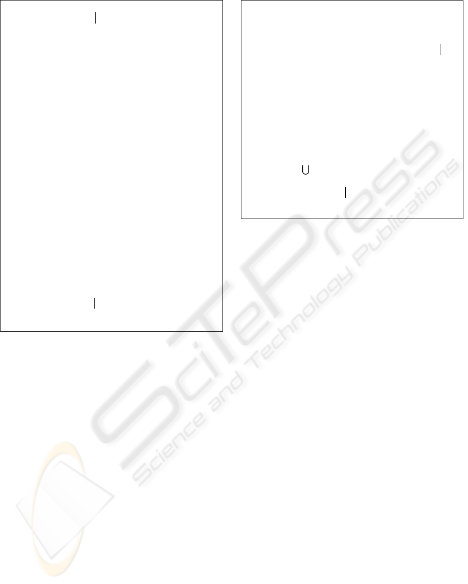
one origin, even if there is more than one. In Figure 4,
the VDT computes that S(q) = {a} and S(r) = {b}.
For p, one of the nearest origins from its 4-neighbors
Figure 4: Pixels a, b and c are object pixels. Pixel p is
the pixel under consideration, q and r are its relevant 4-
neighbors.
is taken. Thus S(p) ∈ S(q) ∪ S(r) = {a, b}, while
the actual nearest origin is S(p) = {c}. This situa-
tion occurs when there are three object pixels a, b, c
so that k~aqk < k~cqk, k
~
brk < k~crk, k~cpk < k~apk,
and k~cpk < k
~
bpk, i.e., when the hatched area con-
tains a grid point. Mullikin proposes, in his VDT, to
store all nearest origins, and additionally all origins
at a distance within a certain tolerance . Essentially,
VDT computes origin sets as defined in Equation (2).
Mullikin shows that an exact distance transform is ob-
tained when ≥
√
D/D, where D is the number of
spatial dimensions. This result can also be used for
the other methods discussed in this paper.
The VDT computes tolerance-based origin sets
only as a means to compute exact DTs. Mullikin
does not detail on the accuracy of the origin sets
themselves in (Mullikin, 1992). Moreover, he uses
only 4-neighborhoods as these are sufficient for exact
Euclidean distances. We extended VDT to also use
8-neighborhoods (see pseudo code in Fig. 5). These
are useful for improving the origin set accuracy, as
shown in Table 2. The pseudo code can be found in
Figure 5. VDT is compared to the other methods in
Section 8.
6 EUCLIDEAN TFT
The FMTFT visits points in the order of the in-
accurate FMM distances (Sec. 4). Although this
keeps the original FMM advantage of using differ-
ent speed functions, an erroneous propagation order
potentially influences the distance and origin set ac-
curacy (Sec. 1). The idea comes thus naturally to
design an ordered propagation FT which visits the
points in order of the accurately computed distances.
We present the pseudo code of this new method,
called Euclidean TFT, in Figure 6. The neighbor-
hood size s (line 15) and tolerance (line 17) have
the same meaning as for the FMTFT and VDT dis-
VISAPP 2006 - IMAGE FORMATION AND PROCESSING
110
1: for each p ∈ δΩ do
2: S(p) ← {q ∈ δΩ kq −pk ≤ }
3: end for
4: for y from 0 to N − 1 do
5: for x from 0 to M − 1 do
6: update( (x,y), (x-1,y-1) ) if s = 8
7: update( (x,y), (x,y-1) )
8: update( (x,y), (x+1, y-1) ) if s = 8
9: update( (x,y), (x-1, y) )
10: end for
11: for x from M − 1 downto 0 do
12: update( (x,y), (x+1,y) )
13: end for
14: end for
15: for y from N − 1 downto 0 do
16: for x from 0 to M − 1 do
17: update( (x,y), (x-1, y+1) ) if s = 8
18: update( (x,y), (x, y-1) )
19: update( (x,y), (x+1, y+1) ) if s = 8
20: update( (x,y), (x-1, y) )
21: end for
22: for x from M − 1 downto 0 do
23: update( (x,y), (x+1,y) )
24: end for
25: end for
26: procedure update(a,b)
27: if a, b ∈ Ω then
28: C ← S(a) ∪ S(b)
29: D (a) ← min
q∈C
kq − ak
30: S(a) ← {q ∈ C kq −ak ≤ D(a) + }
31: end if
32: end procedure
Figure 5: -Vector Distance Transform (VDT). The image
has dimensions M × N.
cussed above. The initialization is the same as for
the FMTFT, and the propagation is still in the order
of increasing distances. However, where the FMTFT
propagates on D
f
(Fig. 3, line 11), the ETFT prop-
agates on the more accurate distances D (Fig. 6,
line 11).
We found out that the above exact-distance prop-
agation order yielded a comparable speed and accu-
racy, posing no advantage over the FMM order. Thus,
we made the following change. The FMTFT updates
all pixels a ∈ N
U,T
(p) (Fig. 3, line 13); the ETFT
was made to update only pixels a ∈ N
U
(p) (Fig. 6,
line 13). Now the ETFT updates pixels only once,
trading accuracy for speed (see Table 2).
7 GRAPH-SEARCH TFT
The FMTFT and ETFT resemble the graph-search ap-
proach of (Lotufo et al., 2000). However, the graph-
search method propagates only one origin per pixel,
i.e., it is a simple FT. We extended Lotufo’s algo-
rithm to a TFT, so that it can be readily compared
1: for each p ∈ Ω ∪
¯
Ω do
2: if p ∈
¯
Ω then
3: f(p) ← K, D(p) ← −1
4: else if p ∈ δΩ then
5: f(p) ← T, D(p) ← 0, S(p) ← {q ∈ δΩ kq −
pk ≤ }
6: else if p ∈ Ω ∧ p /∈ δΩ then
7: f(p) ← U, D(p) ← ∞
8: end if
9: end for
10: while ∃
q
f(q) = T do
11: p ← arg min
q:f (q)=T
D (q)
12: f(p) ← K
13: for each a ∈ N
U
4
(p) do
14: f(a) ← T
15: C ←
q∈N
K,T
s
(a)∪{a}
(S(q))
16: D (a) ← min
q∈C
kq − ak
17: S(a) ← {q ∈ C kq −ak ≤ D(a) + }
18: end for
19: end while
Figure 6: The Euclidean TFT algorithm (ETFT).
to the FMTFT, VDT, and ETFT methods. Figure 7
gives the pseudo code for this extension, called the
Graph-search TFT (GTFT). Now the differences be-
tween the ETFT and GTFT methods become visible.
While GTFT uses only the flags T and K and updates
all neighboring pixels a of p flagged as T (Fig. 7,
line 13), ETFT also uses the flag U and only updates
these pixels (Fig. 6, line 13). Since there are in gen-
eral less pixels flagged U in ETFT than T in GTFT,
ETFT updates less pixels per iteration. However, the
update of a pixel in ETFT involves more work as all
neighbors of a are used (Fig. 6, line 15), whereas in
GTFT only p is used (Fig. 7, line 14). The running
time differences are detailed in the next section.
8 COMPARISON
Unlike DT methods, the computational complexity
of (T)FT methods depends on the origin set sizes
and is therefore strongly input dependent. For ex-
ample, the center of a circle is a worst case, as its
origin set contains all boundary points. The origin
set size, for points inside convex object-regions, in-
creases with distance to boundary. When updating
a pixel p, the whole candidate origin set for p must
be inspected. For N image pixels, and B bound-
ary pixels, this poses a worst case of O(N
2
log B)
for the three propagation-based methods and O(N
2
)
for VDT. Luckily, average real-world images are far
from this worst case. However, it is difficult to mathe-
matically characterize the average input image. Nev-
ertheless, to give more insight into real-world run-
ning times, we empirically compare all discussed TFT
QUANTITATIVE COMPARISON OF TOLERANCE-BASED FEATURE TRANSFORMS
111
1: for each p ∈ Ω ∪
¯
Ω do
2: if p ∈
¯
Ω then
3: f(p) ← K, D(p) ← −1
4: else if p ∈ δΩ then
5: f(p) ← T, D(p) ← 0, S(p) ← {q ∈ δΩ kq −
pk ≤ }
6: else if p ∈ Ω ∧ p /∈ δΩ then
7: f(p) ← T, D(p) ← ∞
8: end if
9: end for
10: while ∃
q
f(q) = T do
11: p ← arg min
q:f (q)=T
kq − pk
12: f(p) ← K
13: for each a ∈ N
T
s
(p) do
14: C ← S(a) ∪ S(p)
15: D (a) ← min
q∈C
kq − ak
16: S(a) ← {q ∈ C kq −ak ≤ D(a) + }
17: end for
18: end while
Figure 7: The Graph-search TFT algorithm (GTFT).
methods on speed and accuracy of both distances and
origin sets. We use images that are often used as typ-
ical input for image processing algorithms.
We implemented all methods and ran them on a
Pentium IV 3GHz with 1 GB RAM. Some design de-
cisions had to be made here. For the propagation-
based methods (FMTFT, ETFT, GTFT) we used a
priority queue to efficiently find the temporary pixel
at minimum distance to the boundary. Origin sets
are always stored as STL multimaps (Musser and
Saini, 1996) containing (distance,origin) pairs, so that
merging two origin sets takes O (n log n) time (as we
must avoid duplicates), while pruning the conserv-
ative set takes O(log n). To prevent floating point
precision problems when performing Statement (4),
it is needed to evaluate kq − pk ≤ D(p) + + τ
instead, where τ is larger than the minimum repre-
sentable difference between two floating point num-
bers. However, τ must be chosen smaller than
1
2
min
p,q ,r∈Ω
k~pqk − k~prk
: half of the minimum
difference between two distances that can occur on
the grid. Alternatively, integer arithmetic can be used
when the equations were rewritten. In our experi-
ments, the use of τ improved the accuracy by two
orders of magnitude.
Table 2 compares the distances D
m
and origin sets
S
m
produced by the methods m to the exact distances
D
e
and origins S
e
, calculated using a brute-force ap-
proach. The table shows measurements on the ‘leaf’
image, and cumulative measurements on 10 differ-
ent images. The considered methods are the FMM,
FMTFT, GTFT, VDT, and ETFT. We do not con-
sider the AFMM Star, as it is a simple FT. For all
methods, except the FMM, we ran the 4 and 8 neigh-
borhood variants, and used 4 different tolerances: 0,
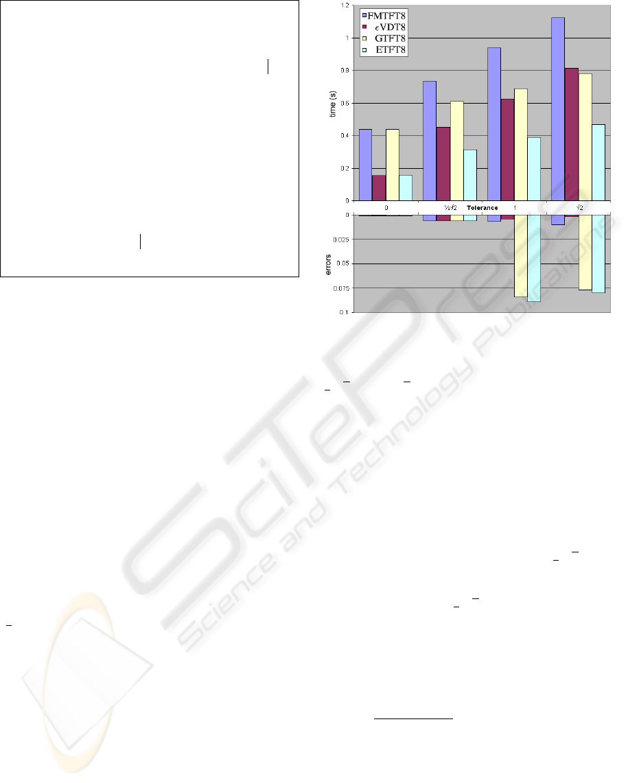
Figure 9: Timings and relative error (e
r
) of the 8-
neighborhood variants for the ‘leaf’ image.
1
2
√
2, 1, and
√
2. For the FMM, we used only the first-
order distance gradient approximation (as mentioned
in Sec. 2), which needs just the 4-neighborhood. The
variants are denoted as, e.g., FMTFT4 0 for the Fast
Marching TFT using a 4-neighborhood and zero tol-
erance.
Table 2 shows that the distance errors decrease by
increasing either the neighborhood size s or the toler-
ance . As previously noted, increasing the neighbor-
hood size does not always eliminate all errors. Indeed,
all methods produce one error for the leaf image with
s = 8 and = 0. As predicted, using =
1
2
√
2 elimi-
nates all errors for all methods; higher tolerances are
not useful for computing exact distances. Finally, our
novel method ETFT4
1
2
√
2 is the fastest of all con-
sidered methods.
We next examine the accuracy of the computed ori-
gin sets. We compare origin sets by comparing the av-
erage relative differences between a method’s origins
and the exact (brute-force method) origins, denoted in
column ‘ ¯e
r
’. Let the relative error e
r
of a pixel p be
e
r
(p) =
|S
m
(p)|−|S
e
(p)|
|S
e
(p)|
, then, ¯e
r
is the average of e
r
over all pixels p ∈ Ω. The tolerance is not only a
means to compute exact distances, but is also a user
parameter for computing origin sets. Unlike for dis-
tances, relaxing the tolerance increases the errors for
origin sets. Indeed, it is more difficult to identify all
origins that are within D(p) + for higher . Note
that, by construction, S
m
⊆ S
e
, i.e., origins are never
falsely identified. It can only happen that S
m
is not
complete. For > 0, none of the considered methods
VISAPP 2006 - IMAGE FORMATION AND PROCESSING
112

Table 2: In each row: distances D
m
and origin sets S
m
of method m are compared to the exact distances D
e
and origins
S
e
. Left table: method comparison for the ‘leaf’ image. Right table: cumulative comparison of 10 different images. For
distances (D), we show: the number of erroneous pixels (#e), maximum distance error (max e = max
p
|D
m
(p) −D
e
(p)|),
and average distance error ¯e. For origins (S) we show: the number of pixels for which origin counts are different (#e), and
the average relative error ¯e
r
(see text). Timings are denoted in seconds in column t.
D
m
S
m
D
m
S
m
method m #e max e ¯e #e ¯e
r
t Σ#e Σ#e Σ ¯e
r
Σt
FMM 29381 1.01 0.25 170 0.182% 0.31 147938 1202 0.306% 1.47
FMTFT4 0 18 0.19 0.00 320 0.309% 0.31 674 2792 0.576% 1.58
VDT4 0 22 0.19 0.00 218 0.147% 0.13 685 1889 0.304% 0.64
GTFT4 0 22 0.19 0.00 218 0.147% 0.28 685 1891 0.304% 1.28
ETFT4 0 18 0.19 0.00 317 0.304% 0.13 674 2779 0.573% 0.61
FMTFT8 0 1 0.04 0.00 1 0.001% 0.44 144 267 0.072% 2.09
VDT8 0 1 0.04 0.00 1 0.001% 0.16 145 217 0.054% 0.89
GTFT8 0 1 0.04 0.00 1 0.001% 0.44 145 217 0.054% 2.11
ETFT8 0 1 0.04 0.00 1 0.001% 0.16 144 267 0.072% 0.83
FMTFT4
1
2
√
2 0 0.00 0.00 12428 8.452% 0.50 0 35828 3.888% 3.31
VDT4
1
2
√
2 0 0.00 0.00 540 0.125% 0.31 0 2285 0.093% 2.60
GTFT4
1
2
√
2 0 0.00 0.00 31835 23.120% 0.31 0 128672 21.655% 1.89
ETFT4
1
2
√
2 0 0.00 0.00 26914 16.744% 0.19 0 146949 17.137% 1.19
FMTFT8
1
2
√
2 0 0.00 0.00 34 0.006% 0.73 0 412 0.010% 5.16
VDT8
1
2
√
2 0 0.00 0.00 34 0.006% 0.45 0 392 0.009% 3.86
GTFT8
1
2
√
2 0 0.00 0.00 34 0.006% 0.61 0 392 0.009% 3.59
ETFT8
1
2
√
2 0 0.00 0.00 34 0.006% 0.31 0 410 0.010% 2.20
FMTFT4 1 0 0.00 0.00 7674 3.879% 0.66 0 23854 1.835% 4.39
VDT4 1 0 0.00 0.00 162 0.025% 0.42 0 415 0.023% 3.42
GTFT4 1 0 0.00 0.00 22306 11.805% 0.41 0 107543 13.522% 2.53
ETFT4 1 0 0.00 0.00 15916 7.763% 0.25 0 89708 8.963% 1.76
FMTFT8 1 0 0.00 0.00 44 0.007% 0.94 0 151 0.004% 6.63
VDT8 1 0 0.00 0.00 32 0.004% 0.63 0 89 0.002% 5.24
GTFT8 1 0 0.00 0.00 250 0.084% 0.69 0 1611 0.164% 4.36
ETFT8 1 0 0.00 0.00 284 0.089% 0.39 0 1404 0.129% 2.81
FMTFT4
√
2 0 0.00 0.00 17654 8.083% 0.75 0 59747 4.562% 5.27
VDT4
√
2 0 0.00 0.00 142 0.018% 0.55 0 286 0.015% 4.77
GTFT4
√
2 0 0.00 0.00 36718 19.525% 0.42 0 169396 20.611% 2.64
ETFT4
√
2 0 0.00 0.00 29446 14.286% 0.30 0 152655 14.830% 1.98
FMTFT8
√
2 0 0.00 0.00 43 0.010% 1.13 0 165 0.005% 8.39
VDT8
√
2 0 0.00 0.00 16 0.002% 0.81 0 27 0.000% 6.81
GTFT8
√
2 0 0.00 0.00 273 0.077% 0.78 0 1105 0.124% 5.25
ETFT8
√
2 0 0.00 0.00 279 0.080% 0.47 0 1130 0.157% 3.58
Figure 8: Locations of origin errors for the leaf image, =
√
2. From left to right: FMTFT8, VDT8, GTFT8, and ETFT8.
The boundary and erroneous pixels are thickened for better display.
QUANTITATIVE COMPARISON OF TOLERANCE-BASED FEATURE TRANSFORMS
113

deliver the complete origin set, although some have
only a few erroneous pixels. From Table 2, we see that
the 8-neighborhood variants have the best accuracy
(< 0.1%). Of these, ETFT8 is the fastest (see also
Fig. 9). For applications needing maximum accuracy,
VDT8 is the method of choice. Although VDT8 has
a better complexity, it is probably slower because of
the hidden time constant: the image is scanned twice.
Finally, we illustrate the locations of the pixels with
erroneous origin sets for the leaf image in Figure 8.
9 CONCLUSION
In this paper, we both analyzed and extended sev-
eral distance and feature transform methods for bi-
nary images. Our goal was to provide a guide for
practitioners in the field for choosing the best method
that meets application-specific accuracy, speed, and
output completeness criteria. First, we perfected the
existing simple-FT method AFMM to deliver more
accurate results (AFMM Star, Sec. 3). We next ex-
tended this method to a new tolerance-based feature
transform, FMTFT, that allows e.g. overcoming un-
desired sampling effects when computing skeletons
(Sec. 4). Next, we discussed three other easy-to-
implement TFT methods: the existing VDT (Sec. 5),
the new ETFT (Sec. 6), and the GTFT extension of
Lotufo’s graph-searching method (Sec. 7).
For computing exact distances, ETFT4
1
2
√
2 is the
fastest of the considered methods. Although there
are other, faster, exact DT methods, e.g. (Meijster
et al., 2000), the ETFT4
1
2
√
2 can accommodate
early distance-based termination and has a simple im-
plementation (cf. Fig. 6). For computing origin sets,
all methods produce fairly accurate results (< 0.1%
errors) for tolerances even up to
√
2. VDT8 is the
most accurate, while ETFT8 is the fastest. Finally,
FMTFT8 is still useful, as it is the only considered
method that can handle different speed functions.
We next intend to extend our TFT methods to 3D
and investigate their relative performance and accu-
racy. This should be rather straightforward, as all
considered methods either do not depend on dimen-
sion (FMTFT, GTFT, ETFT) or have equivalents in
higher dimensions (FMM, VDT). Next, we plan to
apply the TFT methods to compute robust skeletons
of 3D and higher dimensional objects.
ACKNOWLEDGEMENTS
This work was supported by the Netherlands Organ-
isation for Scientific Research (NWO) under grant
number 612.065.414.
REFERENCES
Costa, L. and Cesar, Jr, R. (2001). Shape analysis and clas-
sification. CRC Press.
Cuisenaire, O. (1999). Distance transformations: fast al-
gorithms and applications to medical image process-
ing. PhD thesis, Universit
´
e catholique de Louvain,
Belgium.
Danielsson, P.-E. (1980). Euclidean distance mapping.
In Computer Graphics and Image Processing, vol-
ume 14, pages 227–248.
Foskey, M., Lin, M., and Manocha, D. (2003). Efficient
computation of a simplified medial axis. In Proc. of
the 8th ACM symposium on Solid modeling and appli-
cations, pages 96–107. ACM Press.
Lotufo, T., Falcao, A., and Zampirolli, F. (2000). Fast
euclidean distance transform using a graph-search al-
gorithm. In Proc. of the 13th Brazilian Symp. on
Comp. Graph. and Image Proc., pages 269–275.
Meijster, A., Roerdink, J., and Hesselink, W. (2000). A
general algorithm for computing distance transforms
in linear time. In Goutsias, J., Vincent, L., and
Bloomberg, D., editors, Mathematical Morphology
and its Applications to Image and Signal Processing,
pages 331–340. Kluwer.
Mullikin, J. (1992). The vector distance transform in two
and three dimensions. In CVGIP: Graphical Mod-
els and Image Processing, volume 54, pages 526–535.
Kluwer.
Musser, D. and Saini, S. (1996). STL tutorial and reference
guide: C++ programming with the standard template
library. Addison-Wesley Professional Computing Se-
ries.
Ogniewicz, R. and K
¨
ubler, O. (1995). Hierarchic voronoi
skeletons. In Pattern Recognition, volume 28, pages
343–359.
Ragnemalm, I. (1992). Neighborhoods for distance trans-
formations using ordered propagation. In CVGIP: Im-
age Understanding, volume 56, pages 399–409.
Sethian, J. (1999). Level set methods and fast marching
methods. Cambridge University Press, 2nd edition.
Strzodka, R. and Telea, A. (2004). Generalized distance
transforms and skeletons in graphics hardware. In
Proc. of EG/IEEE TCVG Symposium on Visualization
(VisSym ’04), pages 221–230.
Telea, A. and van Wijk, J. (2002). An augmented fast
marching method for computing skeletons and center-
lines. In Proc. of the symposium on Data Visualisa-
tion, pages 251–259.
Telea, A. and Vilanova, A. (2003). A robust level-set algo-
rithm for centerline extraction. In Proc. of the sympo-
sium on Data Visualisation, pages 185–194.
Ye, Q. (2003). The signed euclidean distance transform and
its applications. In International Conference on Pat-
tern Recognition, volume 1, pages 495–499.
VISAPP 2006 - IMAGE FORMATION AND PROCESSING
114
