
ROBUST CAMERA MOTION ESTIMATION IN VIDEO SEQUENCES
Xiaobo An, Xueying Qin, Guofeng Zhang,Wei Chen, Hujun Bao
State Key Lab of CAD & CG, Zhejiang University
China, 310058
Keywords:
Motion Estimation.
Abstract:
Camera motion estimation of video sequences requires robust recovery of camera parameters and is a cum-
bersome task concerning arbitrarily complex scenes in video sequences. In this paper, we present a novel
algorithm for robust and accurate estimation of camera motion. We insert a virtual frame between each pair
of consecutive frames, through which the in-between camera motion is decomposed into two separate compo-
nents, i.e., pure rotation and pure translation. Given matched feature points between two frames, one point set
corresponding to the far scene is chosen, which is used to estimate initial camera motion. We further refine
it recursively by a non-linear optimizer, yielding the final camera motion parameters. Our approach achieves
accurate estimation of camera motion and avoids instability of camera tracking. We demonstrate high stabil-
ity, accuracy and performance of our algorithm with a set of augmented reality applications based on acquired
video sequences.
1 INTRODUCTION
Structure and motion problem is one of the most
important research topics in the past decade. Gen-
erally speaking, there are two steps to fulfill this
task. Feature tracking(Zivkovic and van der Heij-
den, 2002; Georgescu and Meer, 2004) is first per-
formed to find the correspondences between two
images. Based on the correspondences, camera
tracking and/or structure reconstruction can be ac-
complished by applying two-view(epipolar geome-
try)(Zhang, 1998; Zhang and Loop, 2001) or multi-
view (trilinear tensor) (Shashua and Werman, 1995;
Stein and Shashua, 2000; Sharp et al., 2004; Hart-
ley and Zisserman, 2000) based techniques. Many
methods aim to estimate structure and motion by us-
ing special constraints, like lines, features on planes,
etc.(Johansson, 1990; Alon and Sclaroff, 2000; Polle-
feys et al., 2004). These constraints are typically too
strong to be applied in general scenes. Kalman fil-
ter based methods (Azarbayejani and Pentland, 1995)
can be used either for the estimation of initial solu-
tion or for bundle adjustment involved in the camera
motion estimation. However, the linear update intro-
duced by Kalman filter is not optimal for highly non-
linear structure and motion problem.
Structure and motion estimation algorithms are
known to be far away from perfect. First, the ac-
curacy of traditional feature tracking methods usu-
ally does not meet the practical requirements, be-
cause they may fail to produce correct matches as-
cribing to inter-occlusions, intersections, moving ob-
jects, large motions or ambiguities. Although some
outlier rejection techniques (Zhang, 1998) are intro-
duced to address this problem, they never promise
to pick out all outliers. Second, the effects caused
by the camera rotation and translation may interfere
with each other. When the number of unknown pa-
rameters increases, the stability tends to drop dramat-
ically(MacLean, 1999), especially when the epipo-
lar geometry is ill-posed due to small camera motion.
Third, the widely used non-linear optimization tech-
niques often get stuck in local minima (Kahl and Hey-
den, 2001). Small camera motion and noisy feature
correspondences aggravate this problem. Therefore,
the choice of the initial value for an optimizer is very
crucial.
For outdoor scenes taken by a hand-held video
camera, robust camera motion estimation is of great
importance. One typical example is Augmented Re-
ality (AR) that has been widely used in many appli-
cations such as environmental assessments (Qin et al.,
294
An X., Qin X., Zhang G., Chen W. and Bao H. (2006).
ROBUST CAMERA MOTION ESTIMATION IN VIDEO SEQUENCES.
In Proceedings of the First International Conference on Computer Vision Theory and Applications, pages 294-302
DOI: 10.5220/0001361702940302
Copyright
c
SciTePress

2002) and archeology (Cornelis et al., 2001; Pollefeys
et al., 2004). When virtual objects are located on the
background scenes, an observer is very sensitive to
the accuracy of camera parameters and hence accu-
rate estimation of camera motion is very crucial in
AR-based applications.
The contributions of this paper improve upon pre-
vious approaches in several aspects. First, our ap-
proach does not impose any constraints on scenes.
This makes our approach inherently suitable for gen-
eral scenes. Second, our approach eliminates the high
correlation between the camera rotation and transla-
tion by treating them separately. And the estimation
process involves five parameters of unknowns with-
out any redundancy. In addition, correct estimation of
camera translation direction can be easily achieved,
which is regarded as a key but intractable problem in
camera motion estimation. In consequence, no spe-
cial optimizer is needed for computing precise para-
meters of camera motion.
The remainder of this paper is organized as fol-
lows. After a brief introduction on related work in
Section 2, a conceptual overview is given in Section
3. In Section 4 we present the proposed algorithm for
two consecutive frames. Optimization over continu-
ous frames of a video sequence is introduced in Sec-
tion 5. Experiments results and discussions are de-
scribed in Section 6. Finally, we conclude the whole
paper in Section 7.
2 BASIC STRUCTURE OF A
SCRIPT
Many efforts have been put on robust camera motion
estimation. Traditional methods try to recover the
camera motion by calculating the fundamental ma-
trix or the essential matrix, which usually includes
seven degrees of freedom. Whereas, camera motion
has actually five degrees of freedom. Researchers
have focused on the robust determination of epipolar
geometry(Zhang, 1998; Zhang and Loop, 2001) by
minimizing the epipolar errors. The epipolar errors
of correspondences can be made much less than one
pixel(Zhang and Loop, 2001). However, this does not
lead to a small 3D projection error and accurate cam-
era motion(Chen et al., 2003). Wang and Tsui (Wang
and Tsui, 2000) report that the resultant rotation ma-
trix and translation vector could be quite unstable.
Structure from motion focuses on the recovery of
3D models contained in the scenes. Pollefeys et
al.(Pollefeys et al., 2004) propose an elegant ap-
proach to recover structure and motion simultane-
ously. Two key frames which exhibit obvious mo-
tion are chosen to compute camera motion, and ini-
tial 3D models of the targets are constructed. Subse-
quently, relative camera motion at any frame between
these two key frames is obtained. Additional refine-
ments on both structure and motion are performed for
each frame. This method is hard to deal with gen-
eral scenes because it makes use of the affine-model
based on two assumptions, i.e., frames can be di-
vided into multiple subregions in which all points are
coplanar and these subregions do not change orders
in the video sequence. Obviously, these assumptions
no longer hold for scenes containing inter-occlusions
and intersections objects.
Some researchers try to calculate the camera
translation separately (Jepson and Heeger, 1991;
MacLean, 1999). One technique named ”subspace
methods” generates constraints perpendicular to the
translation vector of camera motion, and is feasible
for the recovery of the translation vector. Recently,
Nist´er et al. (Nist
´
er, 2004) points out that the epipo-
lar based method exploiting seven or eight pairs of
matched points may result in inaccurate camera para-
meters. They instead propose to compute the essential
matrix with only five pairs of point correspondences,
achieving minimal redundancy. With the computed
essential matrix, the camera motion can be estimated
using SVD algorithm. This indirect approach is dif-
ferent from ours, which evaluates camera motion di-
rectly.
Typically, an efficient optimization process is re-
quired to achieve more stable results over the video
sequence. This kind of refinement is often referred
as bundle adjustment technique(Wong and Chang,
2004). It is shown that the bundle adjustment tech-
nique can also be applied to drift removal (Cornelis
et al., 2004).
3 VARIABLES
For each video sequence, we assume that the intrin-
sic parameters of the camera are unchanged and have
been calibrated in advance. The study on camera mo-
tion estimation can be concentrated on the compu-
tation of extrinsic camera parameters in each frame,
which is composed of one rotation matrix R and one
translation vector T.
As an overview, we first introduce the camera
model briefly in conventional notations. We denote a
3D point and its projective depth by homogenous co-
ordinates X =(X, Y, Z, 1)
and λ. The homogenous
coordinates u =(x, y, 1)
specify its projection in a
2D image. The 3 × 3 rotation matrix and triple trans-
lation vector are defined as R = {r
k
,k =0, ..., 8}
and T =(t
0
,t
1
,t
2
)
, respectively. Throughout this
paper we will use the subscript i to denote the frame
number, the subscript j to specify the index number
of feature points, E for the essential matrix, and I for
ROBUST CAMERA MOTION ESTIMATION IN VIDEO SEQUENCES
295
the identity matrix.
For a video sequence containing N frames, we de-
fine the first frame as the reference frame. The camera
model is built upon the camera coordinate system cor-
responding to the reference frame. Suppose that the
number of 3D points is M, and the camera motion
from the first frame to the ith frame is denoted by P
i
with P
0
=(I|0), R
i
and T
i
are the rotation matrix
and translation vector from frame i to frame i +1,it
yields:
λ
1
u
1,j
= P
0
X
j
,λ
i
u
i,j
= P
i
X
j
,
λ
i+1
u
i+1,j
=(R
i
|T
i
)P
i
X
j
= P
i+1
X
j
i =1, ..., N, j =1, ..., M
(1)
Our goal is to recover all R
i
and T
i
, i =1, ..., N − 1.
Note that, 3D points X
j
,j =1, ..., M are unknown
variables, while each u
i,j
can be computed by any
efficient feature tracking algorithm.
Given arbitrary two consecutive frames f
i
and
f
i+1
, to simplify the notations, we omit the super-
scripts for all parameters involved in the previous
frame f
i
and use the superscript
for those of f
i+1
.
Hence, for any 3D point X,wehave:
λu = P
0
X,λ
u
=(R|T )X = RX + T (2)
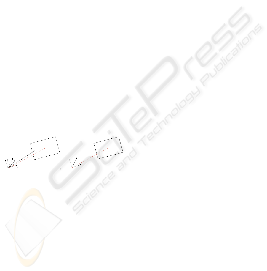
We propose to decompose the camera motion be-
tween f
i
and f
i+1
to pure rotation and pure translation
by inserting a virtual frame f
v
, i.e. f
i
→
R
f
v
→
T
f
i+1
,
through which R and T can be computed separately,
as shown in Figure 1.
The virutal frame
C
Pure rotation
Pure translation
'
The (i+1)th frame
C
The ith frame
Figure 1: A virtual frame is inserted between f
i
and f
i+1
,
based on which the camera motion is decomposed into pure
rotation and translation.
Using the superscript
to specify the parameters
relating to f
v
, it yields:
λ
u
= RX,λ
u
= RX + T = λ
u
+ T
(3)
Note that, the camera motion between f
i
and f
i+1
re-
sults in 2D movement du = u
− u for each point
u in f
i
. Similar to the decomposition of the camera
motion, du can be viewed as the sum of two parts,
namely, du
r
= u
− u, which is the 2D movement
caused by pure rotation, and du
t
= u
−u
, which is
the 2D movement due to pure translation, hence:
du =(u
− u)+(u
− u
)=du
r
+ du
t
(4)
Based on this decomposition, we will show how the
camera motion can be recovered precisely in the next
section.
4 CAMERA MOTION
ESTIMATION BETWEEN TWO
CONSECUTIVE FRAMES
Traditional methods usually involve redundant para-
meters and invoke the uncertainty of camera motion
recovery. In contrast, our algorithm estimates the
camera motion defined by five unknown parameters
of R and T directly without redundant parameters. In
addition, we intends to decompose the 2D movement
of each feature point into two parts and estimate them
individually. Consequently, aforementioned correla-
tion between R and T during the computation process
is avoided.
4.1 Movements of the Feature Points
We first analyze the characteristics of the 2D move-
ments of feature points. From Equation (2), we have:
du =
x
− x
y
− y
=
r
0
x+r
1
y+r
2
+t
0
/Z
r
6
x+r
7
y+r
8
+t
2
/Z
− x
r
3
x+r
4
y+r
5
+t
1
/Z
r
6
x+r
7
y+r
8
+t
2
/Z
− y
(5)
There are two extreme cases in the context of cam-
era motion. One is pure rotation, wherein the move-
ment of u is associated with three Euler angles and its
2D homogenous coordinates, while is irrelevant to the
depth of corresponding 3D point. In practice, when
the translation of a camera is very small compared to
the depth of a 3D point, i.e., T/Z1, the 2D
movement of this point approximates to a pure rota-
tion. The other case is pure translation, or say:
λ
u
=(I|0)X + T = λu +
t
0
t
1
t
2
(6)
Thus, we have:
du =
x
− x
y
− y
=
1
λ
t
0
t
1
−
t
2
λ
x
y
(7)
From Equation (7), it is clear that the 2D movement
du is depending on the projective depth λ
.
Since the translation between two consecutive
frames is very small, the 2D movements of near fea-
ture points are more sensitive to the camera transla-
tion than those of far feature points. Enlightened by
this observation, we seek to first compute a set of far
feature points corresponding to the far region and uti-
lize them for stable estimation of R. The far region
can be viewed as a far depth layer.
4.2 Detection of the Far Depth
Layers
The automatic detection of the far depth layer is per-
formed for the first frame. In case that it fails, we
VISAPP 2006 - MOTION, TRACKING AND STEREO VISION
296

can select the far feature points manually for the first
frame. The automatic detection method for the first
frame classifies all feature point pairs by considering
their disparities. The set of points with the length of
disparities larger than some given threshold is called
the max-group. Likewise, the min-group refers to the
set of points with the length of disparities smaller than
another selected threshold. Typically, there are two
circumstances, i.e., either the min-group or the max-
group corresponds to the far depth layer. We compute
the likeness for each circumstance and choose the one
with the larger likeness. Its corresponding region is
regarded as the far depth layer. In our experiments,
this approach produces correct results for all outdoor
scenes.
Note that, the depth layers in a video sequence may
be different from view to view. For example, a far
point in one frame may switch to a near point in an-
other frame. In addition, many feature points may
disappear along the video sequence. Thus, it is neces-
sary to detect the far depth layer for each frame. For
each successive frame, the automatic update of the far
depth layer is performed after the estimation of the
underlying camera motion, as described in Section
4.3 and 4.4. With the recovered camera parameters,
we calculate corresponding 3D point for each feature
point pair. We then re-select far points based on the
depth of feature points, yielding the far depth layer of
current frame.
4.3 Initial Estimation of the Camera
Motion
It is critical to provide good initial estimations that
are close to the ground-truth, because optimization
processes usually lead to locally optimal solutions.
Our solution is based on the assumption that the 2D
movements of the far points in frames are caused al-
most by camera rotation. The reason is that the in-
fluence induced by the camera translation of the far
points is too small to be counted at the beginning. We
adopt the fixed camera model (Qin et al., 2002) to cal-
culate the initial R based on the far depth layer. It
works well between two consecutive frames, where
the camera rotations are quite small.
By subtracting the movement caused by camera ro-
tation, i.e., du
t
= du − du
r
, an initial estimation of
the 2D movement due to the camera translation can
be obtained. We then recover the camera translation
with these 2D movements. More concretely, in order
to obtain precise translation vector, we take into ac-
count two cases of the camera translation. If t
2
=0,
we have:
du
t
=
x
− x
y
− y
=
1
λ
t
0
t
1
(8)
Equation (8) means that the resultant movement is
completely determined by the projective depth. Here,
all 2D movement vectors take the same direction and
different sizes. On the other side, the resultant move-
ment is determined by both projective depth and its
2D location (x, y) if t
2
is nonzero.
In practice, if there is no movement along z, we set
the translation vector as T =(t
0
,t
1
, 0), and T =
(t
0
,t
1
, 1) contrariwise. Under pure translation, we
have E =[T ]
×
. Suppose that l
= Eu =(l
1
,l
2
,l
3
)
and l = E
u =(l
1
,l
2
,l
3
)
, we can calculate an ini-
tial translation T by minimizing Equation (9) using
LMeds method(Zhang, 1998; Chen et al., 2003):
min
T
j
1
√
l
2
1
+l
2
2
+
1
√
l
2
1
+l
2
2
u
[T ]
×
u
(9)
The recovered R and T are rough estimated values be-
cause the movements of the far points are not caused
entirely by a pure rotation. Therefore, both of du
t
and du
r
are inaccurate. To refine these results, an ad-
ditional iterative optimization is required. Neverthe-
less, it is worthy mentioning that R and T are good
enough as the initial values for the optimization. The
reason for this is that the camera translation between
two consecutive frames is small enough compared to
the depth of the far points. Moreover, the camera
translation direction is of great importance in the op-
timizing process. Fortunately, the 2D movements of
the feature points in frames are well suitable for the
estimation of the direction of T, as demonstrated by
our experiments.
4.4 Iterative Estimation of Camera
Motion
In this section, we use the superscript number to count
the iteration step. We call the handled two frames as
the previous and successive frames. By means of the
initial estimations of R and T , i.e., R
(0)
and T
(0)
,
the 3D coordinates X
(0)
j
j =1, ..., M of all feature
points are recovered. For the sake of simplicity, we
explain our algorithm by taking the kth iteration as
our example. We assume that R
(k)
, T
(k)
and X
(k)
j
are known. We employ a two-step iterative method to
optimize the initial estimations of R and T .
In the first step, we calculate du
(k+1)
t,j
for all j based
on T
(k)
and X
(k)
j
because the camera motion between
the virtual frame and the successive frame is pure
translation. Subsequently, we subtract the movement
caused by translation, yielding more precise du
(k+1)
r,j
,
i.e., du
(k+1)
r,j
= du
j
− du
(k+1)
t,j
. Finally, we compute
R
(k+1)
by minimizing the re-projected difference D
r
:
D
r
=
M
j=0
(u
j
−
˜
u
j
2
+ u
j
−
˜
u
j
2
), (10)
ROBUST CAMERA MOTION ESTIMATION IN VIDEO SEQUENCES
297

where
˜
u
j
and
˜
u
j
denote the re-projected points in the
previous frame and the inserted virtual frame.
We begin the second step by fixing R
(k+1)
.We
re-calculate the 2D movement of all feature points
caused by the camera rotation, i.e., du
(k+1)
r,j
. The 2D
movements caused by the camera translation are up-
dated correspondingly by du
(k+1)
t,j
= du
j
−du
(k+1)
r,j
.
Then, we compute T
(k+1)
by minimizing the re-
projected error D
t
:
D
t
=
M
j=0
(u
j
−
˜
u
j
2
+ u
j
−
˜
u
j
2
), (11)
where
˜
u
j
denotes the re-projected point in the succes-
sive frame. With R
(k+1)
and T
(k+1)
, X
(k+1)
j
can be
achieved conveniently.
We perform this two-step optimization recursively
till the sum of two errors are below some user-
determined threshold :
D
t
+ D
r
< (12)
The nonlinear optimization is accomplished by
Levenberg-Marquardt algorithm. Note that, we pick
out outliers again based on projection error and the
recovered 3D points after each iteration. On advan-
tage pf our method is that only two or three unknowns
are evaluated in each step. The iterative optimization
minimizes the projection errors corresponding to R
and T recursively. This scheme effectively eliminates
the correlation of R and T , and favors robust camera
motion estimation.
5 SPECIAL CONSIDERATIONS
OVER VIDEO SEQUENCE
To achieve robust camera motion estimation over
a video sequence, there are additional cares to be
taken even if all camera motions between consecutive
frames are recovered.
Structure and motion can only be approximated up
to an undetermined similarity, that is, the reconstruc-
tion is subject to arbitrary scaling. Exploiting the fact
that the distance of any two 3D points in the scene
should be fixed, we normalize the translation vector to
obtain a uniform space. More concretely, for each pair
of consecutive frames, we can obtain the 3D coordi-
nates of all feature points based on recovered cam-
era motion, we then compute the distance between
any two 3D points, and optimize a scale which keeps
every distance in the successive frame constant.
On the other hand, bundle adjustment can be car-
ried out to smooth some occasional failed camera
estimation. We first use the recovered camera pa-
rameters between two consecutive frames to evalu-
ate overall camera parameters along the video se-
quence and optimize the overall camera motion by
Levenberg-Marquardt algorithm. We then reconstruct
the scene and get a uniform depth map for the whole
sequence. Next, we use the method similar to that of
Pollefeys etc. (Pollefeys et al., 2004) to refine the in-
between camera parameters between the first and the
last frames. Our experiments show that bundle adjust-
ment is very efficient for normalizing the 3D space of
scenes, smoothing camera motion and removing drift
over the sequence.
6 EXPERIMENTAL RESULTS
AND DISCUSSIONS
We have performed several experiments on both syn-
thetic data sets and real video sequences to examine
the accuracy of our algorithm.
6.1 Synthetic Video Sequences
We first evaluate the performance based on a synthetic
video sequence. We predefine the camera motion for
the entire sequence and choose 300 image points for
the first frame. The correspondence points through
the sequence are calculated from the known camera
motion and their 3D coordinates. Gaussian noise is
added to both x and y image coordinates for all cor-
respondences.
In Table 1, the ground-truth and estimated cam-
era parameters corresponding to R and T by different
methods are compared. The matching errors of fea-
ture points are simulated by a Gaussian noise whose
average is 1.0 pixel. The second and third items list
the results using our method, with and without itera-
tion process(Section 4.4) respectively. It is obvious
that the iterative optimization improves the accuracy
much. The results by means of the Singular Value De-
composition(SVD) of the essential matrix (Wang and
Tsui, 2000) are listed in the fourth item. Surprisingly,
our method outperforms the SVD method even when
no iteration optimization is performed.
Table 2 lists the results of our method under dif-
ferent Gaussian noise sizes. Here, R is represented
by three Euler angles α, β and γ, and p
α
, p
β
and p
γ
denote the percentage of differences between the re-
covered Euler Angles and real ones. The accuracy of
T is measured by the angle difference θ
T
in degrees
between the recovered one and the real one. Row
2-5 show the accuracy of the camera parameters by
means of our method. The numbers listed in Row 6-9
demonstrate the results by Levenberg-Marquardt op-
VISAPP 2006 - MOTION, TRACKING AND STEREO VISION
298

Table 1: Accuracy comparisons of R and T for a synthetic
video sequence.
Real R Real T
0.9999 0.0157 4e-005 9.9752
-0.0157 0.9999 0.0071 -0.5898
7e-005 -0.0071 1.0000 0.4910
R with iteration T with iteration
0.9999 0.0151 3e-005 9.9480
-0.0151 0.9999 0.0073 -0.9022
7e-005 -0.0073 1.0000 0.5621
R without iteration T without iteration
0.9998 0.0179 4e-005 9.9967
-0.0179 0.9998 0.0074 0.3500
8e-005 -0.0074 1.0000 0.1800
R using SVD T using SVD
1.0000 0.0100 4e-005 1.0291
-0.0100 0.9999 0.0057 0.9212
8e-006 -0.0057 1.0000 9.9089
Table 2: Accuracy of camera motion under five noise
sizes. Row 2-5 demonstrate the results using our method.
The results shown in Row 6-9 are achieved by Levenberg-
Marquardt optimizer directly after the initial estimation.
Noise 0.1 0.5 1.0 1.5 2.0
p
α
0.019% 0.080% 0.095% 1.005% 2.800%
p
β
0.017% 0.025% 0.055% 0.750% 2.200%
p
γ
0.002% 0.010% 0.055% 0.095% 0.300%
θ
T
0.7 1.9 3.2 6.7 14.1
p
α
0.045% 0.110% 0.175% 1.520% 3.000%
p
β
0.025% 0.055% 0.130% 1.260% 2.900%
p
γ
0.005% 0.020% 0.150% 0.180% 0.400%
θ
T
3.2 4.6 6.1 13.2 19.0
timizer after the initial estimation of camera motion.
Our method produces more reasonable results.
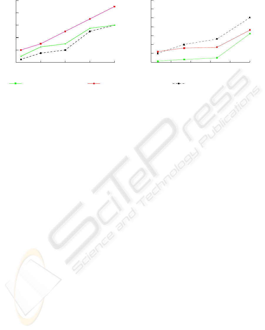
There are two criteria to measure calibration er-
rors. One is the distance from the matched points
to their epipolar lines, called the average epipolar er-
ror. The other one is the average distance between the
re-projected 2D points and the measured 2D points,
called average projection error. We compare both
errors among our method and traditional algorithms
as shown in Figure 2. In Figure 2(a), the average
epipolar error using epipolar based method(Zhang
and Loop, 2001) is slightly smaller than that of our
method. Figure 2(b) demonstrates that our method
is superior to other approaches in the context of the
projection errors. This is because small 2D residual
errors do not correspond to accurate camera parame-
ters as reported in(Chen et al., 2003). In this context,
camera motion estimation methods resulting in small-
est epipolar error are probably not the best choice. In-
stead, the projection error is a better measurement.
6.2 Real Video Sequences
We examine our algorithm on four real video
sequences containing large natural scenes
by integrating a virtual 3D sculpture model
into each video sequence. The intrinsic pa-
rameters are calibrated with OpenCV li-
brary(http://sourceforge.net/projects/opencvlibrary/).
The feature tracking is accomplished based on the
technique introduced in (Georgescu and Meer,
2004). The resultant matching error between two
consecutive frames is less than 1.0 pixel, with some
outliers. Their average projection errors in 20 frames
for each step are illustrated in Figure 3. It is clear that
two-step iteration favors finding a desirable solution
and bundle adjustment increases the stability and
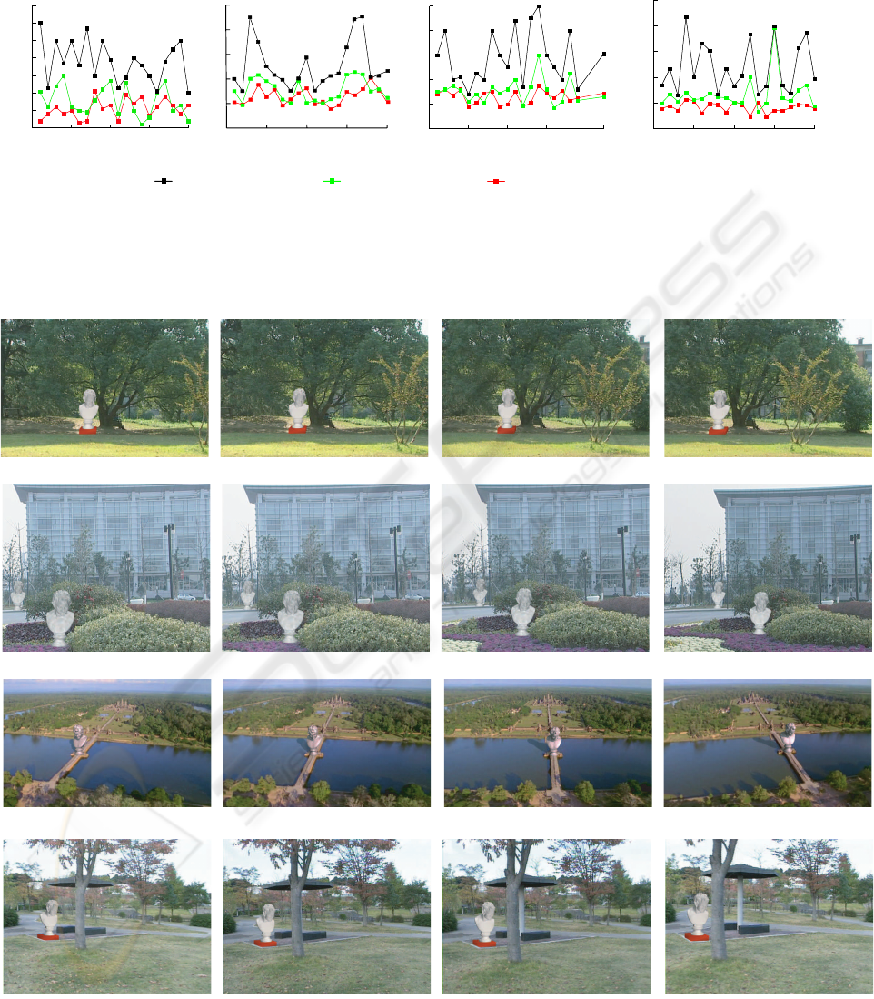
smoothness over a sequence. Figure 4 shows four
representative key frames from each video sequence.
The sequence shown in the top row of Figure
4 demonstrates a case where the translation domi-
nates the camera motion. The camera moves right-
wards and rotates slightly. The scene contains a lot
of intersections and occlusions which makes feature
matching difficult. Traditional algorithms are hard to
achieve precise solutions, especially for T . In con-
trast, our decomposition scheme favors highly accu-
rate recovery of camera parameters as shown in Fig-
ure 3(a).
The second row of Figure 4 shows a scene where
the camera moves backward slowly while rotates. The
2D movements are very small and thus camera esti-
mation is very sensitive to the correspondence error.
Fortunately, the 2D movements of each depth layer
can be grouped correctly by our method, and facil-
itates both depth detection (Section 4.2) and initial
camera estimation (Section 4.3). The average pro-
jection error shown in Figure 3(b) indicates the ro-
bustness of our method even under some occasional
camera dithering.
The scene corresponding to the third row of Figure
4 is captured under a quite complex camera motion.
The camera moves around and focuses on the far spot
(shown in Red) all the time. Neither R nor T is dom-
inant. Nevertheless, our method achieves relative low
average projection error even without bundle adjust-
ment as shown in Figure 3(c).
Among four video sequences, the scene shown in
the last row of Figure 4 has the most complex cam-
era motions. The camera motion exhibits a random-
walk style. Figure 3(d) depicts the average projection
error. Traditional methods result in relatively large
projection errors due to high complexity and discon-
tinuity of the camera motion. In our method, bun-
dle adjustment is very useful for smoothing camera
motion along a video sequence and making uniform
structure, although the average projection error does
not decrease greatly.
ROBUST CAMERA MOTION ESTIMATION IN VIDEO SEQUENCES
299
0.0 0.5 1.0 1.5 2.0
0.0
0.2
0.4
0.6
0.8
1.0
Matching error in pixel
Avergae epipolar error in pixel
Our method with iteration
Our method without iteration
Epipolar geometry method
a)
b)
0.0 0.3 0.6 0.9 1.2 1.5
0.0
0.5
1.0
1.5
2.0
2.5
3.0
3.5
Matching error in pixel
Average projection error in pixel
Figure 2: Comparisons of (a) epipolar errors and (b) projection errors among our method and traditional algorithms.
Our video submission encapsulates all four video
sequences in which a sculpture is composed.
7 CONCLUSIONS AND FUTURE
WORK
We have pursued a robust camera motion estima-
tion method without any assumptions on the scene.
The camera motion between two consecutive frames
are decomposed into pure rotation and pure transla-
tion by inserting a virtual frame. Therefore, the 2D
movements of feature points are separated into two
parts owing to camera rotation and translation respec-
tively. The initial evaluation of the rotation matrix is
achieved by exploiting selected far feature points. The
translation vector is then derived. Since the far fea-
ture points are not infinite far practically, the rotation
matrix and translation vector need to be iteratively re-
fined. Our experiments on both synthetic and real data
demonstrate that our algorithm works well for general
scenes, e.g., scenes containing extreme complicated,
self-intersecting and inter-occluding objects.
Our future work includes improving the algorithm
to work on sequences which include large area of
moving object, moving objects detection and track-
ing, etc. In addition, dealing with an arbitrary-length
video sequence is also in our schedule.
ACKNOWLEDGEMENTS
This paper is supported by NSF of China
(Grant No.60373035), 973 program of China
(No.2002CB312104), NSF of China for Innovative
Research Groups (Grant No.60021201) and Spe-
cialized Research Fund for the Doctoral Program of
Higher Education(No.20030335083).
REFERENCES
Alon, J. and Sclaroff, S. (2000). Recursive estimation of
motion and planar structure. In Proceedings of IEEE
Computer Vision and Pattern Recognition, pages 550–
556.
Azarbayejani, A. and Pentland, A. P. (1995). Recursive es-
timation of motion, structure, and focal length. IEEE
Transactions on Pattern Analysis and Machine Intel-
ligence, 17(6):562–575.
Chen, Z., Pears, N., McDermid, J., and Heseltine, T. (2003).
Epipolar estimation under pure camera translation. In
Proceedings of Digital Image Computing: Techniques
and Applications 2003, pages 849–858, Sydney, Aus-
tralia.
Cornelis, K., Pollefeys, M., and Gool, L. V. (2001). Track-
ing based structure and motion recovery for aug-
mented video productions.
Cornelis, K., Verbiest, F., and Gool, L. V. (2004). Drift de-
tection and removal for sequential structure for motion
algorithms. IEEE Transactions on Pattern Analysis
and Machine Intelligence, 26(10):1249–1259.
Georgescu, B. and Meer, P. (2004). Point matching under
large image deformations and illumination changes.
IEEE Transactions on Pattern Analysis and Machine
Intelligence, 26(6):647–688.
Hartley, R. and Zisserman, A. (2000). Multiple view geom-
etry in computer vision. Cambridge University Press.
Jepson, A. D. and Heeger, D. J. (1991). A fast subspace
algorithm for recovering rigid motion. In Proceedings
of IEEE Workshop on Visual Motion, pages 124–131.
Johansson, B. (1990). View synthesis and 3D reconstruc-
tion of piecewise planar scenes using intersection lines
between the planes. In Proceedings of International
Conference on Pattern Recognition 1999, pages 54–
59.
VISAPP 2006 - MOTION, TRACKING AND STEREO VISION
300

Kahl, F. and Heyden, A. (2001). Euclidean reconstruction
and auto-calibration from continuous motion. In Pro-
ceedings of International Conference on Computer Vi-
sion 2001, pages 572–577, Vancouver, Canada.
MacLean, W. J. (1999). Removal of translation bias when
using subspace methods. In Proceedings of Interna-
tional Conference on Computer Vision 1999, pages
753–758.
Nist
´
er, D. (2004). An efficient solution to the five-point
relative pose problem. IEEE Transactions on Pattern
Analysis and Machine Intelligence, 26(6):756–777.
Pollefeys, M., Gool, L. V., Vergauwen, M., Verbiest, F.,
Cornelis, K., Tops, J., and Koch, R. (2004). Vi-
sual modeling with a hand-held camera. International
Journal of Computer Vision, 59(3):207–232.
Qin, X., Nakamae, E., and Tadamura, K. (2002). Automati-
cally compositing still images and landscape video se-
quences. IEEE Computer Graphics and Appliactions,
22(1):68–78.
Sharp, G. C., Lee, S. W., and Wehe, D. K. (2004). Multi-
viewregistration of 3D scenes by minimizing error be-
tween coordinate frames. IEEE Transactions on Pat-
tern Analysis and Machine Intelligence, 26(8):1037–
1050.
Shashua, A. and Werman, M. (1995). Trilinearity of three
perspective views and its associated tensor. In Pro-
ceedings of International Conference on Computer Vi-
sion 1995, pages 920–925.
Stein, G. P. and Shashua, A. (2000). Model-based bright-
ness constraints: On direct estimation of structure and
motion. IEEE Transactions on Pattern Analysis and
Machine Intelligence, 22(9):992–1025.
Wang, W. and Tsui, H. T. (2000). An SVD decomposition
of essential matrix with eight solutions for the relative
positions of two perspective cameras. In Proceedings
of the International Conference on Pattern Recogni-
tion 2000, pages 1362–1365, Barcelona, Spain.
Wong, K. H. and Chang, M. M. Y. (2004). 3D model recon-
struction by constrained bundle adjustment. In Pro-
ceedings of the 17th International Conference on Pat-
tern Recognition, pages 902–905.
Zhang, Z. (1998). Determining the epipolar geometry and
its uncertainty: A review. International Journal of
Computer Vision, 27(2):161–198.
Zhang, Z. and Loop, C. (2001). Estimating the fundamen-
tal matrix by transforming image points in projective
space. Computer Vision and Image Understanding,
82(2):174–180.
Zivkovic, Z. and van der Heijden, F. (2002). Better fea-
tures to track by estimating the tracking convergence
region. In Proceedings of IEEE International Confer-
ence on Pattern Recognition 2002, pages 635–638.
ROBUST CAMERA MOTION ESTIMATION IN VIDEO SEQUENCES
301
After bundle adjustment
After iteration
Before iteration
Frame No.
Frame No.
0 5 10 15 20
0.0
0.2
0.4
0.6
0.8
1.0
Frame No.
0 5 10 15 20
0.1
0.2
0.3
0.4
0.5
0.6
0.7
0.8
Frame No.
Average projection Hrror in pixel
a) b)
c)
d)
Average projection error in pixel
Average projection error in pixel
Average projection error in pixel
Figure 3: Average projection errors of four video sequences.
The first frame
The first frame
The first frame
The first frame
The 41th frame
The 91th frame
The 100th frame
The 31th frame
The 141th frame
The 95th frame
The 50th frame
The 100th frame
The 141th frame
The 33th frame
The 68th frame
The 65th frame
Figure 4: Key frames of four sequences where virtual objects are composed.
VISAPP 2006 - MOTION, TRACKING AND STEREO VISION
302
