A NOVEL ASYMMETRIC VARIANCE-BASED HYPOTHESIS

TEST FOR A DIFFICULT SURVEILLANCE PROBLEM

Dalton Rosario

Army Research Laboratory, 2800 Powder Mill Road, Adelphi, MD, 20783, U.S.A.

Keywords: Anomaly detection, Asymmetric hypothesis test, Hyperspectral imagery

.

Abstract: Local anomaly detectors have become quite popular for applications requiring hyperspectral (HS) target

detection in natural clutter background assisted by an image analyst. Their popularity may be attributed to

the simplicity of the algorithms designed to function as such. A disadvantage of using such detectors,

however, is that they often produce an intolerable high number of detections per scene, which—according to

image analysts—becomes a nuisance rather than an aiding tool. We present an effective local anomaly

detector for HS data. The new detector exploits a notion of indirect comparison between two sets of samples

and is free from distribution assumptions. The notion led us to derive a compact solution for a variance test,

in which, under the null hypothesis, the detector’s performance converges to a known distribution.

Experimental results using both simulated multivariate data and real HS data are presented to illustrate the

effectiveness of this detector over five known alternative techniques

.

1 INTRODUCTION

Local anomaly detectors have become quite popular

for applications requiring target detection in natural

clutter background assisted by an image analyst.

Their popularity may have been attributed to the

simplicity built into these algorithms. Detectors from

this family search the pixels of sensor imagery for

rare pixels whose information significantly differs

from the local background. These detectors then are

poised to find both known and unknown target

types. The disadvantage, however, is that they often

produce an intolerable high number of detections per

scene, which according to image analysts becomes a

nuisance rather than an aiding tool.

Recently, the use of hyperspectral sensor

imagery (HSI) has also gained renewed attention in

the target detection community. Its popularity over

broadband imagery (e.g., forward looking infrared)

is due to the fact that these passive sensors

simultaneously record images for hundreds of

contiguous and narrowly spaced regions of the

electromagnetic spectrum. Each image corresponds

to the same ground scene, thus creating a cube of

images that contain both spatial and spectral

information about the objects and backgrounds in

the scene. HSI has been used in various fields

including geology, urban planning, geography,

cartography, and the military (Schowengerdt, 1997).

A host of different types of anomaly detectors and

their performances in HSI are discussed in

(Manolakis, 2002), (Kwon, 2003), (Schweizer,

2000), and (Yu, 1997).

Our recent interest has been on a general idea for

anomaly detection, one that performs a comparison

between two observations by an indirect means. The

implementation of this idea has the potential to

preserve the number of meaningful anomaly

detections and to significantly reduce the number of

meaningless anomaly detections. Fig. 1 clarifies this

principle.

Comparing two samples from digitized imagery

often yields three particular study cases: (1) results

from two relatively pure samples belonging to the

same population (Y in Fig. 1), (2) results from two

relatively pure samples belonging to distinct

populations (X and Y), and (3) results from a

composite sample (XY mixture) and a single

component (e.g., Y) sample of that mixture. For

example, a comparison between two observations

sampled from the same tree class falls under case 1,

a comparison between a sample from a ground

vehicle and a sample from a local grass falls under

case 2, and a comparison between a sample with two

components (e.g., a tree & its shadow) and a sample

277

Rosario D. (2006).

A NOVEL ASYMMETRIC VARIANCE-BASED HYPOTHESIS TEST FOR A DIFFICULT SURVEILLANCE PROBLEM.

In Proceedings of the First International Conference on Computer Vision Theory and Applications, pages 277-284

DOI: 10.5220/0001360802770284

Copyright

c

 SciTePress

from one of these components (e.g., shadow) falls

under case 3.

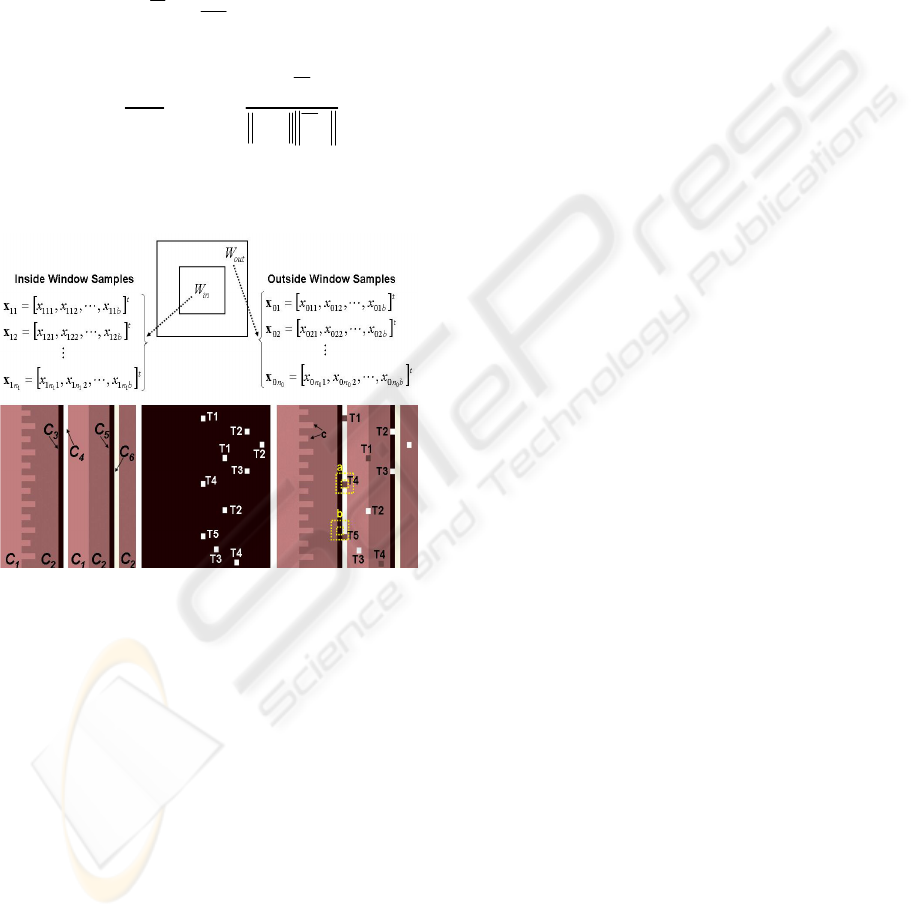
Using a conventional dual rectangular window

(see Fig. 2) to sample locally the imagery, one can

readily verify that case 3 appears quite often and is

arguably responsible for generating a high number

of nuisance detections. The reason is that region

discontinuities are abundant in scene imagery. Local

anomaly detectors based on conventional statistical

methods tend to declare a spectral sample near a

transition of spectral class regions as a local

anomaly. This declaration is correct in the statistical

sense, but also unfortunate, because a local anomaly

detector seems to behave more like an edge detector.

F

Figure 1: The number of nuisance detections may be

significantly reduced by comparing, instead, the union of

candidate samples to one of the candidates. Another

advantage of using this principle is that the number of

meaningful detections is preserved.

We can convert this weakness to strength by

comparing in some form the union of the two

samples to one of the individual observations. Fig. 1

depicts the notion of this indirect approach and its

relevance to comparing two samples. Using this

notion, it is plausible that results for cases 1 and 2

would be unaffected in the statistical sense, but that

results for case 3 would be affected, as shown,

because the construction of a new sample (consisting

of both XY and Y) merely adds more evidence about

Y, making the original composite sample XY a softer

anomaly in respect to the combined sample XYY.

The focus in this paper is to propose a compact

anomaly detector that exploits the principle of

indirect comparison depicted in Fig 1. This new

detector is based on a nonparametric model and has

an asymptotic behavior of the chi square distribution

with 1 degree of freedom. For convenience, this

detector will be referred to as the Asymmetric

Variance Test (AVT) detector.

This paper is organized as follows: Section 2

formulates the technical problem. Section 3 proposes

the AVT detector. Section 4 describes alternative

techniques. Section 5 compares results between the

AVT detector and alternative techniques using

simulated multivariate data and real hyperspectral

(HS) data. Section 5 concludes the paper.

2 PROBLEM FORMULATION

Let B be the clutter background of a simulated

multispectral cube having size r x c x b. Let B

consist of highly correlated but distinct multivariate

random samples of multiple homogeneous classes C

k

(k = 1, …, n

c

).

Now consider a dual rectangular window, as

shown in Fig. 2 (top) and in Fig 2 (bottom) as dotted

boxes at positions a and b, separating the local area

into two regions—the inner window region (W

in

) and

the outer window region (W

out

). This dual window

will slides concentrically across the area r x c in

each simulated cube, such that, at each discrete

position in the imagery, multivariate vector samples

[

]

t

x

pbppp

xxx

020100

,,, L=

(p = 1, … n

0

) that are

viewed within W

out

will be compared in some form

to multivariate vector samples

[

]

t

x

qbqqq

xxx

121111

,,, L=

(q = 1, … n

1

) that are

viewed within W

in

. The size of the dual window is

set such that the W

in

encloses a target sized region

and the W

out

includes its surrounding region. If the

dual window is placed within a spatially

homogeneous region consisting of similar types of

materials, such as natural backgrounds, the statistical

characteristics of samples that are observed within

W

in

and W

out

will be similar to each other. Samples

within W

in

and W

out

will contain significantly

different statistical features, if the dual window is

centered on a region where a target, for instance, is

surrounded by its local background. Use of

appropriate cutoff thresholds on anomaly detectors’

outputs would allow most targets to be detected as

local anomalies, but unfortunately a high number of

detections is attributed to background responses.

A proportionally sized dual rectangular window

with respect to the cubes’ sizes is shown at different

positions on B, see Fig. 2 (bottom). Depending on

the detection technique being used, these

multivariate samples

p0

x

and

q1

x

will be

transformed into two sequences

(

)

0

0010

, ,

n

xxx L

=

and

(

)

1

1111

, ,

n

xxx L=

for

comparison. This transformation is discussed next.

VISAPP 2006 - IMAGE ANALYSIS

278

In general, local spectral information in HS data

is highly correlated, so, to promote statistical

independence, which will be assumed in our model,

we propose a two step pre-processing stage for the

data: (1) differentiate

p0

x

and

q1

x

to yield

[]

t

)1(0010200

,,

−

−−=Δ

bppbppp

xxxx L

(p = 1, …

n

0

) and

[]

t

)1(1111211

,,

−

−−=Δ

bqqbqqq

xxxx L

(q

= 1, … n

1

), and

1

∑

=

Δ=Δ

k

n

i

ki

k

n

; and (2) apply

the following metric,

⎟

⎠

⎞

⎜

⎝

⎛

ΔΔ

=

ki

k

t

i

ki

x

0

arccos

180

π

(1)

where k = 0,1; the operator || z || denotes the squared

root of z

t

z; and

t

][⋅

denotes the vector transpose

operator.

Cube B TRUTH Cube BT

Figure 2: Training cube

B

, shown as the average of five

planes, will be used to obtain cutoff thresholds for

multiple simulated realizations of testing cube

B

T

, also

shown as the average of five planes. The testing cube is

considered a challenging target background configuration

for conventional anomaly detectors because some of

background stripes’ sizes correspond to the size of the

inside window. The ground truth mask is a binary image,

where bright square rectangles representing values of 1

validate target locations. Targets labelled differently (e.g.,

T1 versus T3) have different statistical characteristics

.

Using (1), let x

0

denote the reference feature

vector, x

1

the test feature vector, and let both vectors

be distributed (~) by unknown joint distributions f

0

and f

1

, respectively, or

(x)

f

x

n 11111

~

),...,(

1

=

(2)

,

~

),...,(

00010

0

(x)

f

x

n

=

(3)

where, n

0

= n

1

in this particular implementation.

The dual window is expected to systematically

slide across the imagery and at each location will

pose this question: Do x

0

and x

1

belong to the same

population, or class, in the feature space? If the

answer is no, the test sample will be labelled as an

anomaly with respect to its surroundings at that

location. Random vectors x

0

and x

1

are inputs to the

model discussed next.

3 PROPOSED DETECTOR

We propose in this section the asymmetric variance

test (AVT) anomaly detector. Let random variables

x

0

and x

1

be observed according to the model

,

~

),...,(

11111

1

(x)

g

iid

x

n

=

(4)

,

~

),...,(

00010

0

(x)g iid

x

n

=

(5)

where, x

0

(test sample of size n

1

) and x

1

(reference

sample of size n

0

) are independent, g

1

and g

0

are

unknown, and

, ,

2

1111

∞<=

=

σ

μ

jj

xVarEx

(6)

, ,

2

0000

∞<=

=

σ

μ

jj

xVarEx

(7)

(

)

.

2

0

2

00

∞<=

−

ζ

μ

j

xVar

(8)

Now, consider the null hypothesis

()

.0 :

2

00

>=

ττσ

H

(9)

In (9), we would like to test the hypothesis that

the variance from a reference sample is equal to an

arbitrary positive value. At a first glance, the null

hypothesis does not seem too effective, as a

discriminant feature, because

τ

can take any

positive value, and additionally the variance, as a

discriminant feature, does not account for the mean,

which itself can be another discriminant feature.

However, one can cleverly incorporate the

indirect comparison approach discussed earlier to

test (9), designing in the process a rather effective

anomaly detector. A solution follows.

Let the combined sample be represented by

(

)

(

)

,,...,,,...,,...,

10

1110011 nnn

xxxxttt

=

≡

(10)

where, n = n

1

+n

2

, and lets assume that its

components have the same variance, i.e.,

(

)

∞<=

2

u

k

tVar

σ

. The last assumption may not be

satisfied for all t, but would certainly be satisfied

when x

0

and x

1

are sampled from the same

A NOVEL ASYMMETRIC VARIANCE-BASED HYPOTHESIS TEST FOR A DIFFICULT SURVEILLANCE

PROBLEM

279

population, in which case one could set

2

ˆ

u

στ

=

in

(9), where

2

ˆ

u

σ

estimates

2

u

σ

.

Denoting the symbol

>>

as much greater then,

and

≈

as approximately equal to, the implications of

setting

2

ˆ

u

στ

=

for the study cases shown in Fig. 1

are as follows:

Case 1:

Yx ∈

0

,

Yx ∈

1

, thus,

2

0

2

ˆ

σσ

≈

u

(non-

anomaly).

Case 2:

Xx ∈

0

,

Yx ∈

1

, thus,

2

0

2

ˆ

σσ

>>

u

(strong

anomaly, especially for tight distributions having

μ

0

significantly different from

μ

1

).

Case 3:

XYx ∈

0

,

Yx

∈

1

, thus,

2

0

2

ˆ

σσ

<

u

or

2

0

2

ˆ

σσ

≈

u

(softer anomaly, as the union

10

U xx

merely adds more evidence about Y, retaining the

overall characteristics of the original mixture x

0

).

Without the Normality assumption in (4) and (5),

deriving a test for the null hypothesis in (9) can be

quite difficult. But as we anticipate a relatively large

sample size in HSI, we shall rely on the central limit

theorem (CLT) (Casella, 1990) to design the new

detector.

Using the weak law of large numbers (WLLL),

see for instance (Casella, 1990), the set of

parameters

()

2

00

,

σμ

can be estimated by the

following consistent estimators:

(

)

2

00

, sx

,

respectively, where

()

.

1

,

00

1

0

2

00

2

0

1

0

∑∑

==

−

==

n

j

n

j

n

xx

s

n

x

(11)

Following (11), under general regularity

conditions and using the denotations in (4), CLT

ensures that the random variable z

1

, below,

converges in law to the standard Normal distribution

[N(0,1)], as the sample size

0

n

increases, or

).1,0(

0

2

0

22

0

01

N

s

nz

n

o

⎯⎯⎯→⎯

∞→

−

=

ζ

σ

(12)

To estimate

2

0

ζ

using a consistent estimator

(

)

2

0

ˆ

ζ

, consider this rationale: Let

()

2

00

μϑ

−=

jj

x

and note that, based on (7)

and (8),

(

)

2

0

σϑ

=

j

E

and

(

)

.

2

0

ζϑ

=

j

Var

A

consistent estimator of

(

)

j

Var

ϑ

then would

qualify for application in (12). An obvious estimator

of

(

)

j

Var

ϑ

is

()

∑

=

−

=

0

1

0

2

1

ˆ

n

j

n

V

ϑϑ

ϑ

, where

ϑ

is the sample average using all

j

ϑ

’s. Notice that

ϑ

V

ˆ

can be also expressed by the following

decomposition

(

)

()

{

}

∑

=

−−

−−−−=

0

1

2

0

2

0

1

0

1

00

)1(

ˆ

n

i

nnnV

σϑσϑ

ϑ

,

where the normalized summation term (which does

not include

ϑ

) tends to

2

0

ζ

in probability by the

WLLN, and the term that includes

ϑ

tends to zero

in probability also by the WLLN. Therefore,

ϑ

V

ˆ

is a

consistent estimator of

2

0

ζ

. In addition, using

results from (11), notice that

2

0

s

is also a consistent

estimator of

(

)

j

E

ϑ

. We then propose the

following consistent estimator of

(

)

[

]

2

0 jj

EE

ϑϑζ

−=

to be:

(

)

[

]

.

1

0

1

0

2

0

2

00

2

0

ˆ

∑

=

−

−−

=

n

j

n

sxx

ζ

(13)

Setting

2

ˆ

u

στ

=

in (9), where

(

)

, , ,

1

ˆ

10

11

2

nnn

n

t

n

tt

n

j

n

j

u

+==

−

=

∑∑

==

σ

(14)

if the null hypothesis in (9) is true, the following

must also be true

).1,0(

ˆ

0

2

0

22

0

02

N

s

nz

n

u

⎯⎯⎯→⎯

∞→

−

=

ζ

σ

(15)

Using properties of the family of chi square

distributions [see, for instance, (Casella, 1990)], the

following are also true under the null hypothesis:

(

)

,

2

1

2

0

2

22

0

2

0

ˆ

χ

ζ

σ

⎯⎯⎯→⎯

∞→

−

==

n

u

AVT

s

nzZ

(16)

where

2

1

χ

is the chi-square probability density

function (pdf) with 1 degree of freedom (dof).

Testing hypothesis H

0

in (9) using (16)

constitutes the AVT anomaly detector. A decision

threshold T can be determined via

∫

∞

=

T

dww ,)(

2

1

αχ

where

α

is the type I error (i.e., the probability of

rejecting H

0

, given that H

0

is true). The user chooses

α

, and for values of Z

AVT

greater then T, hypothesis

H

0

is rejected implying that x

0

and x

1

are most likely

sampled from different populations; hence, they are

VISAPP 2006 - IMAGE ANALYSIS

280

anomalous to each other. Otherwise, they are not

significantly anomalous to each other.

4 ALTERNATIVE APPROACHES

A few comments are made in this section on five

well known alternative techniques, which shall be

used in this paper for comparison purposes. Their

mathematical representations are briefly described

and their references are made to the reader. The

alternative techniques are known as: RX (reed-

xiaoli), DPC (dominant principal component), EST

(eigen separation transform), FLD (Fisher’s linear

discriminant), and ANOVA (analysis of variance).

The RX technique (Yu, 1997), the industry

standard, is based on the generalized likelihood ratio

test and on the assumption that the population

distribution family of both test and reference

samples are multivariate normal. The FLD technique

(Kwon, 2003) is also based on the same assumption,

but differs in its subtleties in answering the question

whether the test and reference samples are drawn

from the same normal distribution. The FLD

technique promotes separation between classes and

variance reduction within each class. The DPC and

EST techniques (Kwon, 2003) are both based on the

same basic idea, i.e., data are projected from their

original high dimensional space onto a significantly

lower dimensional space using a criterion that

promotes highest sample variability within each

domain in this lower dimensional space. Differences

between DPC and EST can be appreciated through

their mathematical representations.

Four of these techniques use multivariate vector

samples as inputs, see Fig. 2 (top). These detectors

are defined as:

()()

outin

1

out

t

outin

xxCxx −−=

−

R

X

Z

, (17)

()

outin

t

in

xxE −=

P

CA

Z

, (18)

()

outin

t

ΔC

xxE −=

E

ST

Z

, (19)

and

(

)

outin

t

/SS

xxE

wb

−=

FLD

Z

, (20)

where

in

x

is a sample mean vector from a set of

inside-window vectors

(i)

in

x

, each having b spectral

bands;

out

x

is similar but sampled from the outside

window

(i)

out

x

;

1

out

C

−

is the inverse sample covariance

using all vectors sampled from the outside window;

t

in

E

is the highest energy eigenvector of the

eigenvector decomposition of the inside-window

covariance;

t

ΔC

E

is the highest positive energy

eigenvector of the eigenvector decomposition of the

covariance difference (inside-widow minus outside-

widow); and

t

wb

/SS

E

is the eigenvector

decomposition of the scatter matrices ratio

1

WB

SS

−

,

where

,))((

))((

1

)()(

1

)()(

∑

=

−−

+−−=

out

in

n

i

t

out

i

out

i

n

i

t

in

i

in

i

xxxx

xxxxS

outout

ininW

(21)

and

,))((

))((

1

)()(

1

)()(

∑

=

−−

+−−=

out

in

n

i

tii

n

i

tii

totalouttotalout

totalintotalinB

xxxx

xxxxS

(22)

where

total

x

is the sample average vector using all of

the samples from the inside and outside windows,

and n

in

and n

out

are the sample size of the inside and

outside windows, respectively. For additional details

on these detectors, see (Kwon, 2003).

Our interest in having a well known method

operating in the same feature space of the new

detector’s feature space motivated us to adapt the

ANOVA method into anomaly detection. In the

context of our discussion, using sequences (4) and

(5) as inputs, the ANOVA detector is defined as

()

2

1

0

2

0

S

xxn

Z

i

ANOVA

∑

=

−

=

(23)

where,

i

x

(i = 0, 1) are the sample means of (4) and

(5), also from (4) and (5)

∑∑

==

=

1

01

i

n

j

i

ij

i

n

x

, (24)

and using a version of (11) for x

1

, the pooled

variance can be defined as

)1()1(

00

2

00

2

10

2

−+−

=

nn

snsn

S

. (25)

To the best of our knowledge, the ANOVA

method was never applied to the problem in context.

A NOVEL ASYMMETRIC VARIANCE-BASED HYPOTHESIS TEST FOR A DIFFICULT SURVEILLANCE

PROBLEM

281

5 COMPARATIVE RESULTS

In this section we describe the implementation and

results for two experiment types, one using

simulated multivariate data and another using real

hyperspectral data.

5.1 Simulated Multivariate Data

Let a background

B

consist of six classes

54321

,,,, CCCCC

and

6

C

, and be constructed

using highly correlated, normally distributed

multivariate samples, as follows

() () ()

,,~ ,,~ ,,~

665544

332211

ΣΣΣ

Σ

ΣΣ

μμμ

μ

NCNCNC

(26)

where, “~” denotes “is distributed as,” and the

parameters in (26) are specified as

⎥

⎦

⎤

⎢

⎣

⎡

=Σ

⎥

⎦

⎤

⎢

⎣

⎡

=

0000.101421.140000.201421.140000.10

1421.140000.202843.280000.201421.14

0000.202843.280000.402843.280000.20

1421.140000.202843.280000.201421.14

000.101421.140000.201421.140000.

10

;

650

660

720

640

630

1

μ

and

300

12

−=

μ

,

780

13

−

=

μ

,

1400

14

+=

μ

, 800

15

−=

μ

, and

2000

36

+=

μ

.

Background configuration

B

was constructed to

form a total volume of 256 x 256 x 5 using

simulated realizations of the six classes, as shown in

Fig 2 (bottom). The column widths of narrow stripes

in

B

were chosen to match the column width of W

in

(inside window), see Fig. 2. For targets, five

different multivariate random variables were

specified,

,4,3,2,1 TTTT

and

5T

; they were

specified as follows:

() () ()

() ()

,,~5 ,,~4

,,~3 ,,~2 ,,~1

54

321

ΞΞ

Ξ

ττ

τ

NTNT

NTNTNT

(27)

where,

600

11

−=

μ

τ

,

2000

12

+=

τ

,

2050

13

+=

τ

, 50

14

+=

τ

,

100

15

+

=

τ

,

and, for simplicity, the correlations imbedded in

Ξ

were all equal to 1, and the variances were all equal

to 100. Targets were constructed to form sub-

volumes of constant space size 9 x 9 x 5 using

simulated realizations as specified in the third

dimension. Samples of

B

T cube were formed by

simulating realizations of

B

and adding (9 x 9 x 5)

subcubes of simulated realizations of

,4,3,2,1 TTTT

and

5T

, as shown in Fig. 2.

Details on the information presented in Table 1

and Fig. 3 are discussed next. In order to estimate

type I and type II errors, a 2 dimensional (2D) mask

was required to validate the spatial location of

targets in the simulated imagery. This mask is binary

and often referred to in the target community as

ground truth, see Fig. 2.

Table 1: Confidence Intervals (95% CI).

Alg Type I Error

95% CI

1.0 – Type II

Error 95% CI

LB UB LB UB

AVT

0.111715

0.011173

0.001400

0.000802

0.000788

0.112103

0.011399

0.001496

0.000817

0.000794

1.000

RX

0.101381

0.009608

0.000851

0.000921

0.000074

0.101805

0.009831

0.000861

0.000923

0.000079

1.000

0.700

0.500

1.000

0.700

0.500

FLD

0.101444

0.010374

0.001120

0.000072

0.000019

0.101535

0.010522

0.001279

0.000112

0.000042

0.667

0.500

0.667

0.500

Anova

0.100254

0.009011

0.000978

0.000077

0.000032

0.103467

0.009827

0.001151

0.000107

0.000050

1.000

0.500

1.000

0.500

EST

0.101303

0.010374

0.001120

0.000072

0.000019

0.101394

0.010522

0.001279

0.000112

0.000042

0.700

0.300

0.700

0.300

DPC

0.101444

0.010374

0.001120

0.000072

0.000019

0.101535

0.010522

0.001279

0.000112

0.000042

0.667

0.500

0.667

0.500

In a nutshell, a detector tests a simulated cube

producing a 2D output surface of real values. A

detector-corresponding cutoff threshold, which is

based on a specified type I error and which is

relevant to the cube’s background excluding targets,

is applied to that surface, such that, pixel values that

are above the threshold and which fall within target

regions, as validated through a corresponding

ground truth mask, are considered a correct target

VISAPP 2006 - IMAGE ANALYSIS

282

detection; otherwise, they are considered a false

detection. These measures can be converted into

type I and type II errors by estimating the probability

of correct target detection, which is equivalent to 1

minus type II error, and by estimating the probability

of false detections, which is equivalent to type I

error.

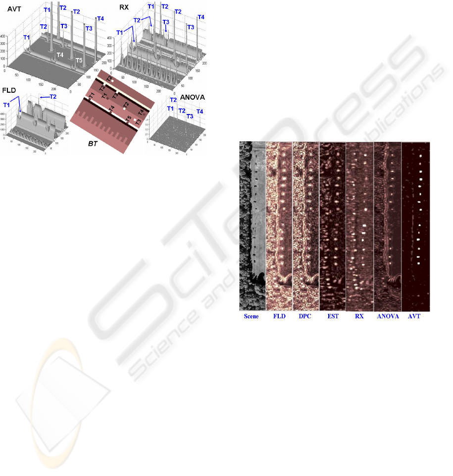
Figure 3: Examples of output surfaces (3D view).

A single simulated realization of the background

configurations

B

was used to obtain cutoff

thresholds based on the following set of desired

Type I errors:

(

)

.10 ,10 ,10 ,10 ,10

54321 −−−−−

=

α

(28)

Type I errors were estimated for each detector

using their corresponding sets of cutoff thresholds

on their output surfaces after testing each detector on

M = 1500 simulated realizations of

B

T .

A generic null hypothesis

0

H

can be stated for

this simulation as follows: At any given location in a

simulated cube, samples observed in

in

W

belong to

the same class of samples observed in

out

W

. The

lower bound (LB) and upper bound (UB) confidence

intervals (CI) are sown in Table 1.

In order to gain a better appreciation for the

differences in performance among different

detectors, see examples output surfaces (3D viewing

perspective) shown in Fig. 3

5.2 Real Hyperspectral Data

Data from the well known Hyperspectral Digital

Imagery Collection Experiment (HYDICE) sensor—

a U.S. Air Force Sensor—were used to compare the

anomaly detectors in this paper. The imagery used is

from the so-called Forest Radiance I (FR-I) dataset

and the spectral average (from 150 bands) of the

sub-cube in reference are shown in Fig. 2 (far left),

as a two dimensional (2D) image. In FR-I, 14

stationary motor vehicles can be observed on sparse

grasses, near a forest in Aberdeen, Maryland, U.S.

The vehicles in FR-I are considered the targets in

this dataset.

Effective local anomaly detectors are expected to

accentuate objects in the scene that are significantly

anomalous to their immediate surroundings and to

suppress noise. Noise in this context also includes

strong responses due to a major transition in local

regions (e.g., grass and shadow).

Examples of 2D output surfaces are shown in

Fig. 4 for the six detectors on HYDICE FR-I data.

These surfaces are displayed in Fig. 4 using the

same colormap (false color), where stronger

intensities depict stronger evidences of local

anomalies.

Figure 4: Decision surfaces for the HYDICE FR-I data,

forest radiance. The intensity of local peaks reflects the

strength of anomaly evidences as seen by different

detectors

.

Fig. 5 presents output surfaces of the industry

standard RX detector and the new AVT detector, as

both these detectors are applied to a difficult

surveillance problem: Ground to Ground (GG)

anomaly detection. The difficulty with this problem

is that, since both a potential target and the viewing

sensor are found approximately at the same ground

elevation, the range between targets and sensor are

unknown, which means that targets’ sizes are

unknown. Additionally, targets may be found in

concealment, e.g., targets in tree shadows.

To handle the GG detection difficulty, the outside

window was eliminated, and two spectral sample

A NOVEL ASYMMETRIC VARIANCE-BASED HYPOTHESIS TEST FOR A DIFFICULT SURVEILLANCE

PROBLEM

283

sets (see square boxes in Fig. 5, top scene) were

made available to the detectors to represent samples

viewed by the outside window. (Notice that in the

GG problem the outside samples are fixed, while the

inside samples will change from location to location,

as the inside window slides across the imagery).

This is a contrast to the high altitude problem

discussed earlier.

SCENES RX AVT

Figure 5. Ground to ground anomaly detection.

The criteria for selecting the fixed outside samples

were based on the abundance level of particular

types of background objects, e.g., in those scenes

shown in Fig. 5, the two most dominant (abundant)

objects in their background are general terrain and

tree leaves, see Fig. 5. The first scene (column 1,

top, in Fig. 5) has two ground vehicles and a person

between these vehicles. The second scene (column

1, center) has a ground vehicle and a person in its

vicinity. The third scene (column 1, bottom) has a

person and a ground vehicle in tree shadows.

So, for a given detector, a set of 100 spectral

samples of terrain and another of tree leaves were

presented as sample references R1 and R2, as they

will be compared to samples W viewed by the inside

window at a give location (i,j) in the imagery.

Denote OUTPUT(i,j) the final output result for this

detector at location (i,j), such that OUTPUT(i,j) is

equal to the minimum between D1 and D2, where

D1 is the detector’s testing result between R1 and W,

and D2 is the detector’s testing results between R2

and W. The OUTPUT surface for the RX and AVT

detectors are shown in Fig. 5, as these detectors

tested the scenes shown in the first column. The

output surfaces show that the AVT anomaly detector

can suppress the background and accentuate the

presence of the ground vehicles and the person in

those scenes, while the industry standard anomaly

detector can not.

6 CONCLUDING REMARKS

We have presented a new local anomaly detector for

hyperspectral sensor imagery. The new detector

(AVT) exploits a notion of indirect comparison

between two sets of samples and yields an

asymptotic behavior, under the null hypothesis, of

the chi-square distribution with 1 degree of freedom.

The AVT detector is simple to implement and has

shown to be very effective accentuating meaningful

local anomalies, while suppressing meaningless

local anomalies in challenging scenes. Results from

this paper elevate the role of anomaly detection from

mere screening (a low impact practical value) to an

effective focus of attention (a high impact practical

value).

REFERENCES

Casella, G., R. L. Berger, 1990. Statistical Inference.

Duxbury Press. Belmont, CA.

Manolakis, D., G. Shaw, 2002. Detection algorithms for

hyperspectral imaging applications. In IEEE Signal

Processing Magazine, pp 29. IEEE Press.

Kwon H., S.Z. Der, and N.M. Nasrabadi, 2003. Adaptive

anomaly detection using subspace separation for

hyperspectral imgery, Opt. Eng., v. 42 (11), pp. 3342-

3351. OE Press.

Schowengerdt, R., 1997. Remote Sensing, Models and

Methods for Image Processing, Academic. San Diego,

2

nd

edition.

Schweizer, S., J. M. F. Moura, 2000. Hyperspectral

Imagery: Clutter Adaptation in Anomaly Detection. In

IEEE Trans. Information Theory, vol. 46, no. 5, pp.

1855-1871. IEEE Press.

Yu, X., L. Hoff, I. Reed, a. Chen, L. Stotts, 1997.

Automatic target detection and recognition in

multiband imagery. In IEEE Tran. Image Processing,

vol. 6, pp. 143-156. IEEE Press

.

VISAPP 2006 - IMAGE ANALYSIS

284