
EBGM VS SUBSPACE PROJECTION FOR FACE RECOGNITION
Andreas Stergiou, Aristodemos Pnevmatikakis, Lazaros Polymenakos
Athens Information Technology
19.5 Km Markopoulou Avenue, P.O. Box 68, Peania, Athens, Greece
Keywords:
Human-Machine Interfaces, Computer Vision, Face Recognition.
Abstract:
Autonomic human-machine interfaces need to determine the user of the machine in a non-obtrusive way. The
identification of the user can be done in many ways, using RF ID tags, the audio stream or the video stream
to name a few. In this paper we focus on the identification of faces from the video stream. In particular, we
compare two different approaches, linear subspace projection from the appearance-based methods, and Elastic
Bunch Graph Matching from the feature-based. Since the intended application is restricted to indoor multi-
camera setups with collaborative users, the deployment scenarios of the recognizer are easily identified. The
comparison of the methods is done using a common test-bed for both methods. The test-bed is exhaustive for
the deployment scenarios we need to consider, leading to the identification of deployment scenarios for which
each method is preferable.
1 INTRODUCTION
The problem of face recognition on still images has
gained much attention over the past years. One of the
main driving factors for this trend is the ever growing
number of applications that an efficient and resilient
recognition technique can address, such as security
systems based on biometric data and user-friendly
human-machine interfaces. Example applications of
the latter are smart rooms (Waibel et al., 2004), where
the presence of humans and their identity is detected
from video feeds. Although many algorithms for face
recognition have been proposed (Zhao et al., 2000;
Brunelli and Poggio, 1993; Turk and Pentland, 1991;
Belhumeur et al., 1997; Gunning and Murphy, 1992;
Wiskott et al., 1999), their performance depends on
how unconstrained the environment is (variations in
pose, illumination, and expression (Belhumeur et al.,
1997; Georghiades et al., 2001; Martinez and Kak,
2001), as well as partial face occlusion (Pentland
et al., 1994)) and on geometric face normalization.
Hence, finding a resilient, all-purpose face recogni-
tion method has proven a tough challenge.
An overview of algorithms for both still- and
video-based face recognition is presented in (Zhao
et al., 2000). A broad categorization of the algo-
rithms is based on the way they treat an image; as
a whole (appearance-based), or in terms of specific,
easily identifiable points on the face (feature-based)
(Brunelli and Poggio, 1993). The most well-known
and studied appearance-based methods are the linear
subspace projection methods: The Eigenface method
(Turk and Pentland, 1991) employs Principal Com-
ponent Analysis (PCA) (Duda et al., 2000), and the
Fisherface method (Belhumeur et al., 1997) couples
that with Linear Discriminant Analysis (LDA) (Duda
et al., 2000) to improve performance. Many vari-
ants of these methods exist (Pentland et al., 1994).
Feature-based approaches include neural networks
(Gunning and Murphy, 1992) and Elastic Bunch
Graph matching (EBGM) (Wiskott et al., 1999).
The aim of this paper is to compare EBGM from
the feature-based approaches with the linear subspace
projection methods from the appearance-based ap-
proaches. The comparison addresses both perfor-
mance and suitability for real-time application. Since
the performance of PCA+LDA under different dis-
tance metrics and number of training images has been
studied (Pnevmatikakis and Polymenakos, 2004; Bev-
eridge and She, 2001), the same is needed for EBGM.
Different identification metrics and number of train-
ing images per subject are utilized to obtain identifi-
cation rates, as well as the ability of EBGM to auto-
matically locate the facial features of interest on the
images. The latter is very important since the overall
system success depends on accurate feature localiza-
tion. This set of experiments establishes a baseline
performance for EBGM. Further experiments are con-
ducted to study the effect on the baseline of varying
image sizes and offsets in the eye positions caused
by imperfect eye detection. The algorithm is im-
plemented in SuSe Linux 9.1 using the RAVL C++
libraries (Christmas and Galambos, 2005) from the
University of Surrey.
131
Stergiou A., Pnevmatikakis A. and Polymenakos L. (2006).
EBGM VS SUBSPACE PROJECTION FOR FACE RECOGNITION.
In Proceedings of the First International Conference on Computer Vision Theory and Applications, pages 131-137
DOI: 10.5220/0001359401310137
Copyright
c
SciTePress

The paper is organized as follows: Section 2 gives
an overview of the EBGM algorithm. Section 3 dis-
cusses the image preprocessing and feature estima-
tion stages. Section 4 describes the face database
used; the baseline EBGM performance is identified
and compared to subspace projection methods. Sec-
tion 5 extends the comparison to different preprocess-
ing schemes and impairments like face size and inac-
curate eye position. Conclusions are drawn in Section
6, along with guidelines for extensions of EBGM.
2 EBGM OVERVIEW
EBGM assumes that the positions of certain facial
features (termed fiducial points in (Wiskott et al.,
1999)) are known for each image in the database.
Information on each face is collected by convolving
the image regions around these fiducial points with
40 complex 2D Gabor kernels. Gabor wavelets are
formed by multiplying a sinusoidal with a Gaussian
function. The Gaussian has a dampening effect, hence
only pixel values near the given fiducial point con-
tribute to the convolution. The resulting 80 coeffi-
cients constitute the Gabor jet for each fiducial point.
The Gabor jets for all fiducial points are grouped in a
graph, the Face Graph, where each jet is a node and
the distances between fiducial points are the weights
on the corresponding vertices. The information in the
Face Graph is all that is needed for recognition; the
image itself is discarded.
All Face Graphs from the training images are com-
bined in a stack-like structure called the Face Bunch
Graph (FBG). Each node of the FBG contains a list of
Gabor jets for the corresponding fiducial point from
all training images, and the vertices are now weighted
with the average distances across the training set. The
exact positions of the fiducial points on the training
images are known.
The positions of the fiducial points in the testing
images are unknown; EBGM estimates them based
on the FBG. Then a Face Graph can be constructed
for each testing image based on the estimated fiducial
point positions. The Face Graph of each testing image
is compared with the FBG to determine the training
image it is most similar with, according to some jet-
based metric.
3 PREPROCESSING, FACE
GRAPHS AND RECOGNITION
Although in principle EBGM can handle some
scale, shift and rotation between the faces, to be
fair in the comparison with the PCA+LDA method
that needs normalization (Pnevmatikakis and Poly-
menakos, 2004), the images are normalized according
to the eye positions. Hence effectively the eye posi-
tions are known also for the testing images.
The normalization involves scaling, rotation and
shifting. The goal is to bring the face at the cen-
ter of the image, rotate and resize it appropriately so
that the eyes are aligned at preselected positions and
at a predefined distance. The normalization parame-
ters (eye coordinates and distance) are selected so that
convolution with even the largest kernel does not ex-
tend outside the image border. Then, the remaining
background is discarded by cropping a rectangular
area around the face. To avoid abrupt intensity vari-
ations at the cropped image border which disrupt the
convolution results, the intensity around the face is
smoothed as proposed in (Bolme, 2003).
The localization of the fiducial points is done in two
steps: initial estimation and refinement. The initial
estimation is based on the positions of the previously
localized face features. Starting with the positions of
the eyes (which are accurately positioned after nor-
malization), an estimate for the position of the n-th
point is obtained by the weighted average
p
n
=
n−1
i=1
w
in
(p
i
+ v
in
)
n−1
i=1
w
in
(1)
where p
i
are the positions of the n-1 previously es-
timated points, v
in
are the average distance vectors
between points i and n from the FBG and w
in
=
e
− v
in
are weighting factors that give more weight
to neighboring features. The sequence of localization
in (Bolme, 2003) is from the eyes radially outwards to
the edge of the face, but our experiments indicate that
this does not improve estimation accuracy; any order
can be used.
The refinement step improves the initial esti-
mate accuracy by using Gabor jet similarity metrics
(Bolme, 2003). The Gabor jet from the initial esti-
mate is compared to all jets in the FBG for that fidu-
cial point. The jet from the FBG with the highest sim-
ilarity is the local expert. The best metric to estimate
the local expert is the Phase Similarity. The local ex-
pert is used for the refinement of the position of the
fiducial point in the testing image, based on the max-
imization of the Displacement Similarity metric as a
function of the displacement between the current jet
of the testing image and its local expert. Four differ-
ent maximization methods are presented in (Wiskott
et al., 1999; Bolme, 2003).
After the fiducial points for a testing image have
been estimated, Gabor jets are extracted from all those
positions to construct the testing Face Graph. The lat-
ter is compared against all training Face Graphs in the
FBG to obtain the identity of the person. A number of
metrics are proposed in (Wiskott et al., 1999; Bolme,
VISAPP 2006 - IMAGE UNDERSTANDING
132

2003) for this comparison.
The simplest metric is to ignore all information in
the Face Graph nodes (the jets) and rely only on that
of the vertices of the Face Graph (the positions of the
fiducial points). A scan across the FBG produces the
member for which the average (across all features)
Euclidean distance from the testing Face Graph is
minimized. This is the Geometry Similarity (GeoS).
Although extremely fast, this metric gives the worst
results by far. This is due to the normalization step
which enforces a uniform distribution of the facial
features across all images, making a successful iden-
tification very difficult even when a very large number
of training images per class are available.
The main drawback of GeoS is that it does not uti-
lize the information about the surrounding areas of the
fiducial points stored in the Gabor jets. The simplest
methods that make use of this information are Magni-
tude Similarity (MS) and Phase Similarity (PS), dis-
cussed in (Wiskott et al., 1999; Bolme, 2003).
A family of more sophisticated metrics is based on
the Displacement Estimation (DE) methods already
discussed. Again we try to find a displacement vec-
tor for the testing Gabor jet that would maximize its
similarity to the corresponding training jet under the
Displacement Similarity metric. The difference now
is that the training jets in the maximization of the met-
ric for all nodes in the testing Face Graph are nodes of
the same member of the FBG and not the local experts
of the testing jets.
4 BASELINE PERFORMANCE
FOR EBGM
For our experiments with EBGM the HumanScan
face database (Jesorsky et al., 2001) is used. This data
set consists of 1,521 grayscale images, corresponding
to 23 different individuals. In some images part of
the face is missing; these images are discarded lead-
ing to a total of 1,373 images belonging to 21 distinct
classes. For each image, the coordinates of 20 hand-
annotated fiducial points are provided. These coordi-
nates are used both in the image preprocessing phase
and in the FBG creation. There is a lot of within-class
diversity, as the database contains images with vari-
ations in illumination, pose (faces are mostly frontal,
but with tilts), expression and occlusions (glasses or
hands). Unfortunately these variations are not per-
formed systematically; hence any given impairment
is not guaranteed to exist across all subjects nor with
the same intensity. This necessitates reporting of the
performance as an average across many runs with dif-
ferent selection of training images.
The goal of the experiments carried out in this sec-
tion is to establish a baseline performance for EBGM
under normal training/testing conditions. By normal
(but not ideal) conditions we define images that are
approximately frontal and with mostly neutral expres-
sions. The only occlusions allowed are normal glasses
(not dark sunglasses) and blinking eyes. Lighting
conditions may vary, but not to the extreme. Hence
the HumanScan database is suitable for the baseline
performance determination. Note that, unless oth-
erwise stated, the eyes have been manually located,
allowing for the testing of the face recognition al-
gorithms in the semi-automatic manner, ignoring the
task of automatic face detection (Yang et al., 2002).
4.1 Refinement of Fiducial Point
Position
Experiments have been carried out to determine the
optimum DE method in terms of accuracy and speed.
Accuracy is measured based on the average RMS es-
timation error across all features and the whole test
image set. Speed is measured as the average time
for fiducial point position estimation per image. The
DEPS (DE Prediction Step) method has no parame-
ters; for the other three the chosen parameter values
are as follows: The maximum number of iterations
for DEPI (DE Predictive Iteration) is 3, 6 and 10, the
grid size for DEGS (DE Grid Search) is 8, 12 and 16
pixels, and the maximum number of search steps for
DELS (DELocal Search) is 10, 25 and 50. The exper-
iments were run on a P4/2.66GHz with 512 MB RAM
under SuSe Linux 9.1. (Bolme, 2003) summarizes the
key characteristics of each of the four DE methods.
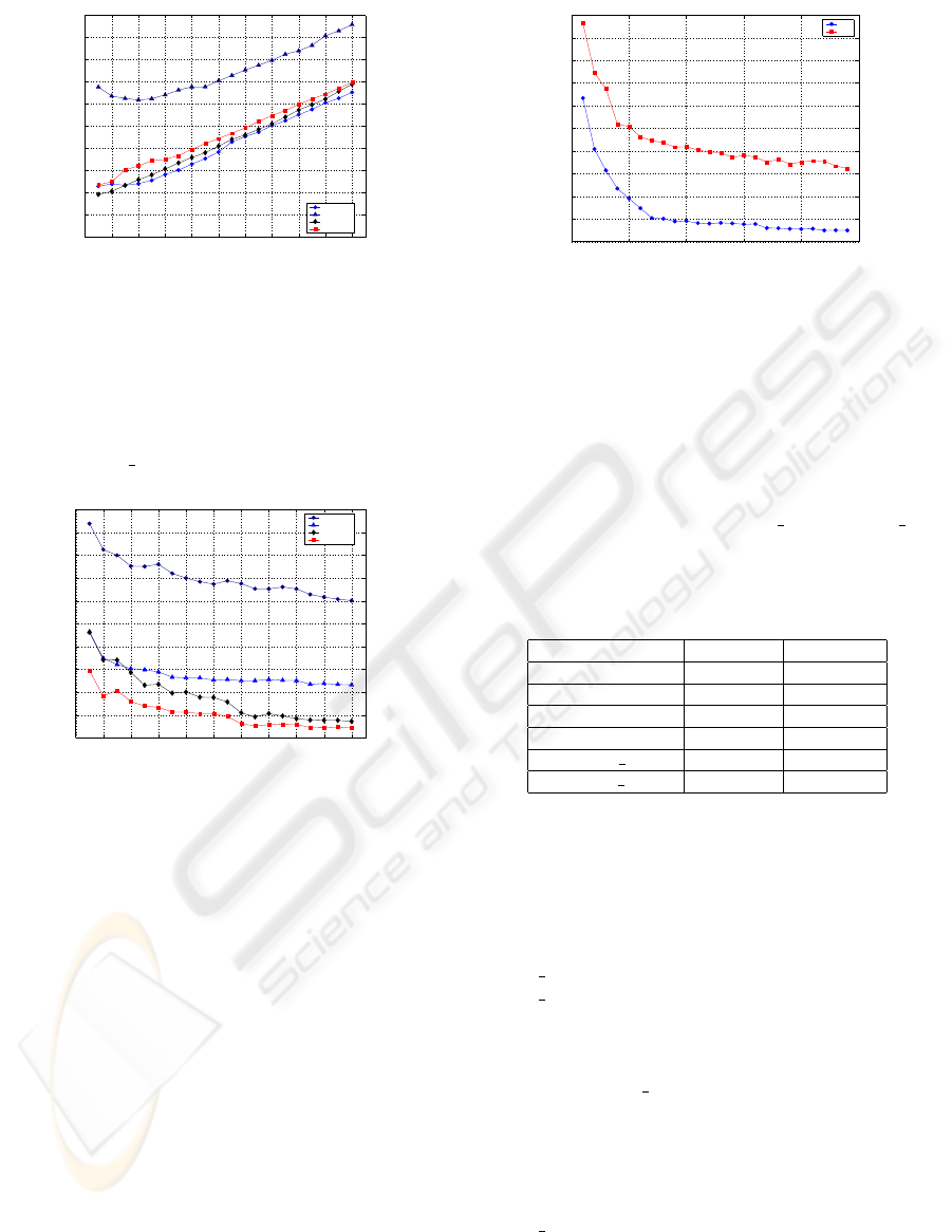
The results in terms of Average Processing Time
(APT) are presented in Figure 1 as a function of the
number of training images per class. For the three
parametric methods, the version that gave the best re-
sults in each case is shown (i.e., DEPI
3, DEGS 8 and
DELS
10). It is clear that DEPI 3 is by far the slowest
DE method, whereas the other three have very small
speed discrepancies. The results are justified as the
bulk of the processing time for feature estimation is
taken up by the convolutions with the Gabor kernels.
Hence DEPS, DEGS
8 and DELS 10 have compa-
rable run times while DEPI
3, which involves more
than one convolution steps, is slower.
The average RMS error over all facial features is
shown in Figure 2. For all three parametric methods,
the parameter value that resulted in faster process-
ing time also gives the most accurate estimation. For
DEPI this is due to the fact that more than three itera-
tions are rarely needed. A similar argument holds for
DELS, while for DEGS the answer lies in the image
normalization. Since the preprocessing stage leads to
a more or less standard face size and orientation, it is
expected that maximization is achieved close to the
initial estimate; therefore increasing the search area
EBGM VS SUBSPACE PROJECTION FOR FACE RECOGNITION
133
0 2 4 6 8 10 12 14 16 18 20
0.2
0.22
0.24
0.26
0.28
0.3
0.32
0.34
0.36
0.38
0.4
Training Images per Class
Time (sec)
Average Feature Estimation Time (All Methods)
DEPS
DEPI_3
DEGS_8
DELS_10
Figure 1: APT for the four DE methods.
has little impact on performance and may even lead
to higher errors if a feature is falsely estimated to lie
farther away from the staring point. Based on its su-
perior performance in terms of RMS error and its fast
run times, DELS
10 is chosen as the DE method.
0 2 4 6 8 10 12 14 16 18 20
4.7
4.8
4.9
5
5.1
5.2
5.3
5.4
5.5
5.6
5.7
Training Images per Class
RMS Error
Average RMS Estimation Error (All Methods)
DEPS
DEPI_3
DEGS_8
DELS_10
Figure 2: Average RMS error across all facial features for
the four DE methods.
4.2 Testing Face Graph Similarity
with FBG
The identification performance of the EBGM algo-
rithm is evaluated based on a variety of Gabor Jet sim-
ilarity metrics, discussed in (Bolme, 2003). For the
local expert identification, the jet phase utilized in the
PS metric yields much better results than the magni-
tude utilized in the MS metric. This is not the case for
determining the FBG member that is most similar to
a testing Face Graph (Wiskott et al., 1999). This fact
is verified in Figure 3, where the performance of both
MS and PS for a single run with between 1 and 24
training images per class is shown. Although a single
run can be misleading, the performance gap between
the two metrics is enough to disregard PS from the
rigorous experimentation that follows.
The use of the DS (Displacement Similarity) metric
for determining the FBG member that is most similar
0 5 10 15 20 2
5
0
5
10
15
20
25
30
35
40
45
50
Training Images per Class
PMC (%)
Identification Performance : MS vs. PS
MS
PS
Figure 3: Comparison of identification performance in
terms of PMC for the MS and PS metrics.
to a testing Face Graph is more promising. From the
four variants, DEPI is not studied because it is exces-
sively slow. The recognition performance in terms of
the Probability of Misclassification (PMC), averaged
over 25 runs with a single training image per class, to-
gether with the identification times, are listed in Table
1 for GeoS, MS, PS, DEPS, DEGS
16 and DELS 25.
Table 1: Comparison of six different similarity metrics
across 25 runs with 1 training image per class. Average
PMC and recognition times are reported.
Similarity Metric PMC (%) Time (ms)
GeoS 86.64 0.148
MS 33.55 4.59
PS 46.61 5.62
DEPS 49.34 13.3
DEGS 16 25.31 458
DELS 25 30.44 44.1
To obtain the baseline performance of EBGM
we extensively experiment with two of the promis-
ing EBGM variants in terms of speed and perfor-
mance, following the general methodology described
in (Pnevmatikakis and Polymenakos, 2005). The MS
is the most promising of the fast variants, whereas
DEGS
16 is the best and slowest variant. The MS and
DEGS
16 variants are compared for different number
of training images per class in Table 2. The PMC and
ID time reported are averages across a large number
of runs with different training and testing subsets. It
is clear that DEGS
16 has consistently superior iden-
tification performance, although the discrepancy be-
tween the two methods is reduced as more training
images per class become available. However, MS
is considerably faster, being able to identify an im-
age in about two orders of magnitude less time than
DEGS
16. We can therefore propose two variants of
the EBGM algorithm according to the metric used
for identification. When identification time is crit-
ical (real-time applications), the best variant is MS,
especially if many training images per class are avail-
VISAPP 2006 - IMAGE UNDERSTANDING
134
able. However, when we are interested in the opti-
mum recognition performance and have no serious
time constraints (off-line applications) the most ap-
propriate variant is definitely DEGS
16. This is con-
sidered the baseline performance for EBGM.
Table 2: Comparison of recognition and speed characteris-
tics between the MS and DEGS
16 metrics.
TPC Runs
PMC (%) ID Time (sec)
MS DEGS 16 MS DEGS 16
2 300 19.79 14.87 0.011 0.957
3 400 13.84 10.24 0.016 1.578
5 400 8.55 6.15 0.032 3.168
10 400 4.84 3.06 0.048 5.164
The baseline performance of EBGM (DEGS 16)
is compared to that of the linear subspace projec-
tion methods. PCA without the 3 eigenvectors that
correspond to the largest eigenvalues (PCAw/o3) is
used as a representative of the unsupervised projec-
tion estimation methods and PCA+LDA for the su-
pervised projection estimation methods (Duda et al.,
2000; Pnevmatikakis and Polymenakos, 2004). The
same experiments have been run for the subspace pro-
jection methods and the averaged PMC is compared
in Figure 4.
1 2 3 4 5 6 7 8 9 10
0
5
10
15
20
25
30
Identification Performance for EBGM and Subspace Projection variants
Training Images per Class
PMC (%)
PCA w/o 3
PCA+LDA
EBGM
Figure 4: Comparison of the average PMC of EBGM
(DEGS
16) and subspace projection methods (PCAw/o3
and PCA+LDA) as a function of the number of training im-
ages per class.
EBGM (DEGS 16) is superior when there is only a
single training image per class, and somewhat better
when there are two. For more than two its perfor-
mance is worse than both subspace projection meth-
ods. Since PCA+LDA is even faster than the MS
EBGM variant, obviously EBGM is not a good choice
when adequate training is available, the conditions are
approximately neutral (in terms of pose illumination
and expression) and the normalization is based on the
ideal eye positions.
5 EFFECT OF IMPAIRMENTS
Having established a baseline identification per-
formance for EBGM under approximately neutral
conditions and having identified it inferior to the
PCA+LDA performance, we now attempt to identify
the effect on that baseline of different preprocessing
and impairments like small image size and imperfect
eye positions. We also extend the comparison with
PCA+LDA, to establish the relative performance of
the two methods under less ideal conditions.
5.1 Effect of Preprocessing
It is argued in (Pnevmatikakis and Polymenakos,
2004; Bolme, 2003) that a different preprocessing
scheme that involves making the images zero-mean
and unit-variance is more appropriate when there are
different illumination conditions in the images. Such
differences exist in HumanScan, hence zero-mean
and unit-variance preprocessing is applied. The faces
in the resulting images are identified using the two
EBGM variants and PCA+LDA.
The results for the two EBGM variants indicate that
there is no clear advantage from the extra preprocess-
ing step. More specifically, in a total of 25 runs using
a single training image per class the average PMC im-
proved only slightly (by 0.24% under MS and 0.03%
under DEGS
16).
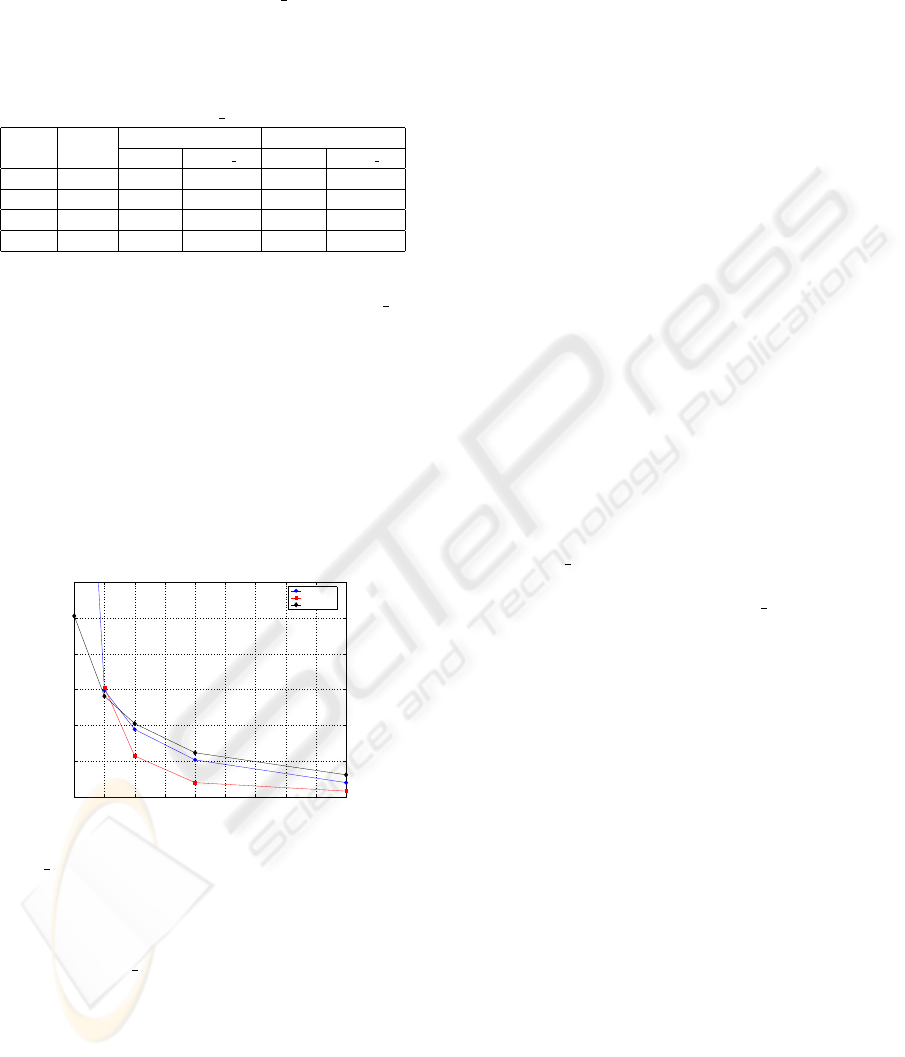
These tests were repeated for 300 runs with 2 train-
ing images per class under the DEGS
16 metric. The
results are depicted as a scatter plot in Figure 5 and
it is obvious that there is again no clear benefit in in-
troducing intensity normalization to the preprocess-
ing step: both the average and standard deviation of
the PMC are practically unaffected. This is not the
case for the PCA+LDA combination. The average
PMC improves, and does so significantly when there
are few training images per class. The individual runs
are also shown as a scatter plot in Figure 5.
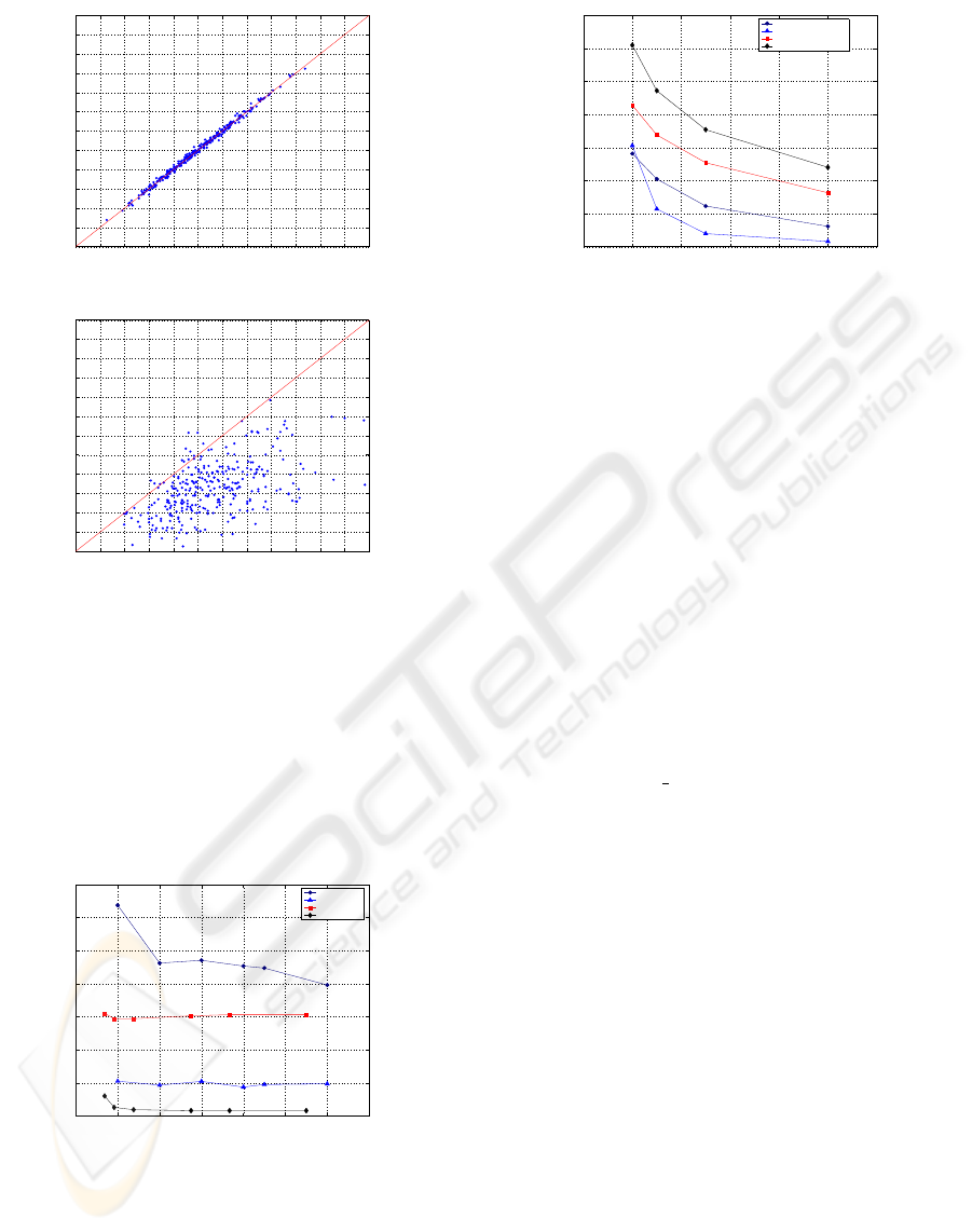
5.2 Effect of Image Size
The resilience of face recognition algorithms to small
face sizes is very important in deployments where
zoom cameras are not available. To investigate the
effect of face size on identification performance, the
HumanScan images are resized and the average PMC
is again reported for the different sizes.
Figure 6 shows the effect of different image sizes
on the recognition performance for a varying num-
ber of training images per class for MS EBGM and
PCA+LDA. We can see that as the image size is re-
duced the PMC increases, which was to be expected
since downscaling smears the facial characteristics
and makes reliable fiducial point location harder. For
EBGM VS SUBSPACE PROJECTION FOR FACE RECOGNITION
135
4 6 8 10 12 14 16 18 20 22 24 26 2
8
4
6
8
10
12
14
16
18
20
22
24
26
28
PMC % (300 runs, 2 TPC, DEGS_16)
w/o Intensity Normalization
with Intensity Normalization
(a)
4 6 8 10 12 14 16 18 20 22 24 26 2
8
4
6
8
10
12
14
16
18
20
22
24
26
28
w/o Intensity Normalization
with Intensity Normalization
PMC % (2 TPC, 300 runs, PCA+LDA)
(b)
Figure 5: Using scatter plots to study the effect of pre-
processing using intensity normalization for EBGM (a) and
PCA+LDA (b).
EBGM, this degradation becomes less noticeable as
more training images per class are used. This indi-
cates that EBGM can withstand changes in scale quite
well if the training set size is large enough.
0 10 20 30 40 50 60 70
0
5
10
15
20
25
30
35
Eye Distance (pixels)
PMC (%)
Effect of Image Size on Identification Performance
MS (2 TPC)
MS (10 TPC)
LDA (2 TPC)
LDA (10 TPC)
Figure 6: Effect of downsizing images for various training
set sizes.
The opposite can be said for PCA+LDA. There the
degradation is minor for 2 training images per class,
but it becomes more noticeable in 10 training images
per class. For extremely small face sizes, the perfor-
mance of EBGM and PCA+LDA is comparable.
0 2 4 6 8 10 1
2
0
5
10
15
20
25
30
35
Effect of Eye Misalignment
Training Images per Class
PMC (%)
EBGM (Perfect Eyes)
LDA (Perfect Eyes)
EBGM (Imperfect Eyes)
LDA (Imperfect Eyes)
Figure 7: Effect of imperfect eye localization for various
training set sizes.
5.3 Effect of Eye Misalignment
The subspace projection methods depend a lot on
proper alignment of the images. Hence normalization
is performed using the annotated eye positions. Un-
fortunately, in automatic face recognition systems the
eye positions can only be estimated by some face de-
tector. These estimates are not always very accurate.
EBGM on the other hand does not in theory demand
accurate eye positions; it takes advantage of the elas-
ticity of the bunch graph to cope with eye misalign-
ments. In this subsection, the eye positions estimated
using an actual eye detector from unpublished work,
which gives an RMS eye position error of 4.12% of
the eye distance, are used to normalize the Human-
Scan images. Then, the recognition performance of
the EBGM (DEGS
16) and the subspace projection
methods (LDA) is compared. The results are depicted
in Figure 7. As expected, EBGM clearly outperforms
PCA+LDA when the eyes are not ideally located.
6 CONCLUSIONS
In this paper we have first established a baseline per-
formance for the EBGM algorithm for face recogni-
tion and compared it to the different subspace pro-
jection methods. We have shown that EBGM can be
used to successfully locate the positions of fiducial
points in novel images, even when only a few training
images per class are contained in the FBG. We then
studied two different metrics used in the recognition
process, leading to two versions of EBGM that could
be used in practice, depending on the particular ap-
plication and its requirements in terms of speed and
recognition accuracy. Finally, we compared EBGM
to subspace projection methods with respect to differ-
ent pre-processing schemes, different image sizes and
imperfect eye localization. Even though PCA+LDA
is faster and better performing than EBGM, we have
VISAPP 2006 - IMAGE UNDERSTANDING
136

established some application scenarios for EBGM.
EBGM seems a very suitable choice when there is
only one training image per class, and a reasonable
choice when there are two. Even for more training
images per class, EBGM should be used when the
images are extremely small, or when the eyes are not
ideally located.
A number of issues are still open. With regard to
identification accuracy, it is clear that we need to uti-
lize more appropriate metrics or enhance the existing
ones. One way to approach this problem is to weigh
the contribution of each fiducial feature by a differ-
ent amount when computing the total similarity over
the whole face. The major obstacle in this case is the
determination of the appropriate weights in a system-
atic way. A simple idea is to weigh each contribution
according to the expected accuracy in estimating the
feature position, so that we bias our decision towards
those fiducial points we have more confidence in.
Another way of improving performance would be
to use a larger number of fiducial points for each
image, by interpolating between the positions of the
known features. For example, 25 original points and
55 interpolated points have been used in (Bolme,
2003) to construct each Face Graph, while we have
used only the 20 points originally defined by Human-
Scan. The main concern here is to avoid using too
many and closely spaced points, as that would de-
grade identification accuracy (Wiskott et al., 1999).
Our early experiments show that adding just one ex-
tra point can improve average performance by about
1%, but some of the tried extra points can degrade
performance by three times as much.
The choice of kernel sizes is also very important as
images are downsized, since the use of smaller ker-
nels would reduce correlation between convolution
results from neighboring jets. Ideally, we would like
to have an algorithm that can dynamically adapt to the
image dimensions and adjust the size and composition
of the kernel set accordingly.
ACKNOWLEDGEMENTS
This work is partly sponsored by the EU under the
Integrated Project CHIL, contract number 506909.
REFERENCES
Belhumeur, P., Hespanha, J., and Kriegman, D. (1997).
Eigenfaces vs. fisherfaces: Recognition using class
specific linear projection. IEEE Trans. Pattern Analy-
sis and Machine Intelligence, 19(7):711–720.
Beveridge, J. and She, K. (2001). Fall 2001 update to CSU
PCA versus PCA+LDA comparison. Technical report,
Colorado State University, Fort Collins, CO.
Bolme, D. S. (2003). Elastic Bunch Graph Matching. Mas-
ter’s thesis, Computer Science Department, Colorado
State University.
Brunelli, R. and Poggio, T. (1993). Face recognition: Fea-
tures versus templates. IEEE Trans. Pattern Analysis
and Machine Intelligence, 15:1042–1052.
Christmas, B. and Galambos, C. (2005). http:
//www.ee.surrey.ac.uk/Research/
VSSP/RavlDoc/share/doc/RAVL/Auto/
Basic/Tree/Ravl.html.
Duda, R., Hart, P., and Stork, D. (2000). Pattern Classifica-
tion. Wiley-Interscience, New York.
Georghiades, A., Belhumeur, P., and Kriegman, D. (2001).
From few to many: Illumination cone models for face
recognition under variable lighting and pose. IEEE
Trans. Pattern Analysis and Machine Intelligence,
23(6):643–660.
Gunning, J. and Murphy, N. (1992). Neural network
based classification using automatically selected fea-
ture sets. IEE Conf. Series 359, pages 29–33.
Jesorsky, O., Kirchberg, K., and Frischholz, R. (2001).
Robust face detection using the Hausdorff distance.
In Audio and Video based Person Authentication -
AVBPA 2001, pages 90–95. Springer.
Martinez, A. and Kak, A. (2001). PCA versus LDA.
IEEE Trans. Pattern Analysis and Machine Intelli-
gence, 23(2):228–233.
Pentland, A., Moghaddam, B., and Starner, T. (1994).
View-based and modular eigenspaces for face recog-
nition. Proc. IEEE Conf. on Comp. Vision & Pattern
Rec., pages 84–91.
Pnevmatikakis, A. and Polymenakos, L. (2004). Compar-
ison of eigenface-based feature vectors under differ-
ent impairments. Int. Conf. Pattern Recognition 2004,
1:296–300.
Pnevmatikakis, A. and Polymenakos, L. (2005). A testing
methodology for face recognition algorithms. In 2nd
Joint Workshop on Multi-Modal Interaction and Re-
lated Machine Learning Algorithms, Edinburgh.
Turk, M. and Pentland, A. (1991). Eigenfaces for recogni-
tion. J. Cognitive Neuroscience, 3:71–86.
Waibel, A., Steusloff, H., and Stiefelhagen, R. (2004).
CHIL - Computers in the Human Interaction Loop.
In 5th International Workshop on Image Analysis for
Multimedia Interactive Services - WIAMIS 2004.
Wiskott, L., Fellous, J.-M., Krueger, N., and von der Mals-
burg, C. (1999). Face recognition by Elastic Bunch
Graph Matching. In Intelligent Biometric Techniques
in Fingerprint and Face Recognition, chapter 11,
pages 355–396. CRC Press.
Yang, M., Kriegman, D., and Ahuja, N. (2002). Detect-
ing faces in images: A survey. IEEE Trans. Pattern
Analysis and Machine Intelligence, 24(1):34–58.
Zhao, W., Chellappa, R., Rosenfeld, A., and Phillips, P.
(2000). Face recognition: A literature survey.
EBGM VS SUBSPACE PROJECTION FOR FACE RECOGNITION
137
