
AN INCREMENTAL WEIGHTED LEAST SQUARES
APPROACH TO SURFACE LIGHTS FIELDS
Greg Coombe, Anselmo Lastra
Department of Computer Science, University of North Carolina at Chapel Hill
Keywords: Image-based rendering, surface light fields, appearance modelling, least-squares approximation.
Abstract: An Image-Based Rendering (IBR) approach to appearance modelling enables the capture of a wide variety
of real physical surfaces with complex reflectance behaviour. The challenges with this approach are
handling the large amount of data, rendering the data efficiently, and previewing the model as it is being
constructed. In this paper, we introduce the Incremental Weighted Least Squares approach to the
representation and rendering of spatially and directionally varying illumination. Each surface patch consists
of a set of Weighted Least Squares (WLS) node centers, which are low-degree polynomial representations
of the anisotropic exitant radiance. During rendering, the representations are combined in a non-linear
fashion to generate a full reconstruction of the exitant radiance. The rendering algorithm is fast, efficient,
and implemented entirely on the GPU. The construction algorithm is incremental, which means that images
are processed as they arrive instead of in the traditional batch fashion. This human-in-the-loop process
enables the user to preview the model as it is being constructed and to adapt to over-sampling and under-
sampling of the surface appearance.
1 INTRODUCTION
A Surface Light Field (SLF) (Wood, 2000) is a
parameterized representation of the exitant radiance
from the surface of a geometric model under a fixed
illumination. SLFs can model arbitrarily complex
surface appearance and can be rendered at real-time
rates. The challenge with SLFs is to find a compact
representation of surface appearance that maintains
the high visual fidelity and rendering rates.
One approach to this problem is to treat it as a
data approximation problem. The exitant radiance at
each surface patch is represented as a function, and
the input images are treated as samples from this
function. Since there are no restrictions imposed on
the geometry of the object or on the camera
locations, the input samples are located at arbitrary
positions. This is an example of a problem known as
scattered data approximation (Wendland, 2005).
(Coombe, 2005) introduced the notion of casual
capture of a SLF by moving a camera around an
object, tracking the camera pose using fiducials, and
incrementally updating the SLF. This enabled the
operator to see the result, add views where needed,
and stop when he or she was satisfied with the result.
However, one difficulty with the matrix factorization
approach is that it requires fully resampled matrices,
and so can be sensitive to missing data from
occlusions and meshing errors.
In this paper we present Incremental Weighted
Least Squares (IWLS), a fast, efficient, and
incremental algorithm for the representation and
rendering of surface light fields. It is a non-linear
polynomial approximation for multi-variate data,
based on the idea of Least Squares polynomial
approximation, which fits scattered data samples to a
set of polynomial basis functions. WLS is similar to
Figure 1: A model of a heart captured with our system
84
Coombe G. and Lastra A. (2006).
AN INCREMENTAL WEIGHTED LEAST SQUARES APPROACH TO SURFACE LIGHTS FIELDS.
In Proceedings of the First International Conference on Computer Graphics Theory and Applications, pages 84-91
DOI: 10.5220/0001358700840091
Copyright
c
SciTePress

piecewise polynomial approximation and splines,
except that the reconstruction is non-linear.
Weighted Least Squares (Wendland, 2005)
generalizes Least Squares by computing a set of
approximations with associated weighting terms.
These weighting terms can be either noise (in
statistics) or distance (in graphics and computational
geometry (Ohtake, 2003)). If we use distance, then
WLS becomes a local approximation method. This
local approximation is extended to a global
approximation by computing the Partition of Unity
(Ohtake, 2003; Shepard, 1968).
This paper offers the following contributions:
• We apply existing mathematical tools such as
the Weighted Least Squares approximation
technique by casting surface light fields as a
scattered data approximation problem.
• We introduce Incremental Weighted Least
Squares, an incremental approach to surface
light field construction that enables
interactive previewing of the reconstruction.
• Using the IWLS representation, we develop a
real-time surface light field rendering
algorithm, implemented on the GPU, which
provides direct feedback about the quality of
the surface light field.
The paper proceeds as follows. We first discuss
previous approaches to light field capture and
representation, including the difference between
batch processing and incremental processing. In
Section 3 we discuss Least Squares fitting and the
generalization to Weighted Least Squares. We then
introduce IWLS and describe how the WLS
representation can be incrementally constructed and
rendered. In Section 4 we discuss implementation
details of the capture and rendering system, and then
present results and conclusion.
2 BACKGROUND
A good overview of the state of the art in material
modelling by image acquisition is provided by the
recent Siggraph course on Material Modelling
(Ramamoorthi, 2002), and the Eurographics State of
the Art Report on Acquisition, Synthesis and
Rendering of Bidirectional Texture Functions
(Mueller, 2004). The choice of representation of this
captured data is crucial for interactive rendering.
(Lensch, 2001) uses the Lafortune representation
(Lafortune, 1997) and clustered samples from
acquired data in order to create spatially-varying
BRDFs. (Gardner, 2003) and (McAllister, 2002)
describe BDRF capture devices and methods for
BRDF representation.
Data-driven representation can be divided into
parametric and non-parametric approaches. A
parametric approach assumes a particular model for
the BRDF (such as the Lafortune model (Lafortune,
1997) used by (McAllister, 2002)). These models
have difficulty representing the wide variety of
objects that occur in real scenes, as observed by
Hawkins in (Yu, 1999).
A non-parametric approach uses the captured
data to estimate the underlying function and makes
few assumptions about the behavior of the
reflectance. Thus non-parametric models are capable
of representing a larger class of surfaces, which
accounts for their recent popularity in image-based
modelling (Chen, 2002; Furukawa, 2002; Matuzik,
2003; Zickler, 2005). Our approach uses a non-
parametric model to represent surface light fields.
2.1 Surface Light Fields
Surface light fields (Wood, 2000) parameterize the
exitant radiance directly on the surface of the model.
This results in a compact representation that enables
the capture and display of complex view-dependent
illumination of real-world objects. This category of
approaches includes view-dependent texture
mapping (Debevec, 1996; Debevec, 1998; Buehler,
2001), which can be implemented with very sparse
and scattered samples, as well as regular
parameterizations of radiance (Levoy, 1996; Gortler,
1996). (Wood, 2000) use a generalization of Vector
Quantization and Principal Component Analysis to
compress surface light fields, and introduce a 2-pass
rendering algorithm that displays compressed light
fields at interactive rates. These functions can be
constructed by using Principal Component Analysis
(Nishino, 1999; Chen, 2002; Coombe, 2005) or non-
linear optimization (Hillesland 2003). The function
parameters can be stored in texture maps and
rendered in real-time (Chen, 2002).
These approaches can suffer from difficulties
stemming from the inherent irregularity of the data.
If they require a complete and regularly sampled set
of data, an expensive resampling step is needed. To
avoid these problems, we treat surface light field
reconstruction as a scattered data approximation
problem (Wendland, 2005). Scattered data
approximation can be used to construct
representations of data values given samples at
arbitrary locations (such as camera locations on a
hemisphere or surface locations on a model).
AN INCREMENTAL WEIGHTED LEAST SQUARES APPROACH TO SURFACE LIGHTS FIELDS
85

A common scattered data approximation
technique uses Radial Basis Functions (RBFs)
(Moody, 1989). (Zickler, 2005) demonstrated the
ability of RBFs to accurately reconstruct sparse
reflectance data. Constructing this approximation
requires a global technique, since every point in the
reconstruction influences every other point. This is a
disadvantage for an incremental algorithm, as every
value must be recomputed when a new sample
arrives. It is also difficult to render efficiently on
graphics hardware, since many RBF algorithms rely
on Fast Multipole Methods to reduce the size of the
computation (Carr, 2001). We would like a method
that has the scattered data representation ability of
RBFs, but without the complex updating and
reconstruction.
2.2 Incremental Methods
Most of the research in image-based modelling has
focused on batch-processing systems. These systems
process the set of images over multiple passes, and
consequently require that the entire set of images be
available. Incorporating additional images into these
models requires recomputing the model from
scratch.
Formulating surface light field construction as an
incremental processing approach avoids these
problems by incrementally constructing the model as
the images become available. (Matusik, 2004) used
this approach with a kd-tree basis system to
progressively refine a radiance model from a fixed
viewpoint. (Schirmacher, 1999) adaptively meshed
the uv and st planes of a light field, and used an error
metric along the triangle edges to determine the
locations of new camera positions. (Coombe, 2005)
used an incremental PCA algorithm to construct
surface light fields in an online fashion, but required
resampling the data for matrix computation.
3 INCREMENTAL WEIGHTED
LEAST SQUARES
IWLS is a technique to incrementally calculate an
approximation to the exitant radiance at each surface
patch given a set of input images. The process is
divided into two parts: constructing the WLS
representation from the incoming images, and
rendering the result. In this section we review Least
Squares fitting and the generalization to Weighted
Least Squares. We then describe how these WLS
representations can be incrementally constructed and
rendered.
3.1 Least Squares Approximation
Least Squares methods are a set of linear
approximation techniques for scattered data. Given a
set of N scalar samples
ℜ∈
i
f
at points
d
i
x ℜ∈
,
we want a globally-defined function f(x) that best
approximates the samples. The goal is to generate
this function f(x) such that the distance between the
scalar data values f
i
and the function evaluated at the
data points f(x
i
) is as small as possible. This is
written as
min f (x
i
) − f
i
i
∑
(Note: this discussion follows the notation of
(Nealen, 2004)). Typically, f(x) is a polynomial of
degree m in d spatial dimensions. The coefficients of
the polynomial are determined by minimizing this
sum. Thus f(x) can be written as
f (x)
=
b(x)
T
c
where b(x) = [b
1
(x) b
2
(x) ... b
k
(x) ]
T
is the
polynomial basis vector and c = [c
1
c
2
... c
k
] is the
unknown coefficient vector. A set of basis functions
b(t) is chosen based on the properties of the data and
the dimensionality.
To determine the coefficient vector c, the
minimization problem is solved by setting the partial
derivatives to zero and solving the resulting system
of linear equations. After rearranging the terms, the
solution is:
[
]
∑∑
−
=
i
ii
i
T
ii
fxbxbxbc )()()(
1
For small matrices, this can be inverted directly.
For larger matrices, there are several common
matrix inversion packages such as BLAS
(Remington, 1996) and TGT. The size of the matrix
to be inverted depends upon the dimensionality d of
the data and the degree k of the polynomial basis.
3.2 Weighted Least Squares
One of the limitations of Least Squares fitting is that
the solution encompasses the entire domain. This
global complexity makes it difficult to handle large
data sets or data sets with local high frequencies. We
would prefer a method that considers samples that
are nearby as more important than samples that are
far away. This can be accomplished by adding a
GRAPP 2006 - COMPUTER GRAPHICS THEORY AND APPLICATIONS
86
distance-weighting term Θ(d) to the Least Squares
minimization. We are now trying to minimize the
function
∑
−−Θ
i
iii
fxfxx )()(min
A common choice for the distance-weighting
basis function Θ(d) is the Wendland function
(Wendland, 1995)
)1
4
()1()(
4
+−=Θ
h
d
h
d
d
which is 1.0 at d = 0, and falls off to zero at the
edges of the support radius h. This function has
compact support, so each sample only affects a small
neighborhood. There are many other weighting
functions that could be used, such as multiquadrics
and thin-plate splines, but some functions have
infinite support and thus must be solved globally.
Instead of evaluating a single global
approximation for all of the data samples, we create
a set of local approximations. These approximations
are associated with a set of points
x
, which are
known as centers. At each of these centers, a low-
degree polynomial approximation is computed using
the distance-weighted samples x
i
in the local
neighborhood.
[]
∑∑
−Θ−Θ=
−
i
iii
i
T
iii
fxbxxxbxbxxxc )()()()()()(
1
We now have a set of local approximations at
each center. During the reconstruction step, we need
to combine these local approximations to form a
global approximation. Since this global function is a
weighted combination of the basis functions, it has
the same continuity properties.
The first step is to determine the m nearby local
approximations that overlap this point and combine
them using a weight based on distance. However,
the functions cannot just be added together, since the
weights may not sum to 1.0. To get the proper
weighting of the local approximations, we use a
technique known as the Partition of Unity (Shepard,
1968), which allows us to extend the local
approximations to cover the entire domain. A new
set of weights Φ(j) are computed by considering all
of the m local approximations that overlap this point
∑
=
Θ
Θ
=Φ
m
i
i
j
j
x
x
x
1
)(
)(
)(
The global approximation of this function is
computed by summing the weighted local
approximations.
∑
=
Φ=
m
j
j
T
j
xcxbxxf
1
)()()()(
The WLS representation allows us to place the
centers
x
wherever we like, but the locations are
fixed. This is in contrast to the Radial Basis
Function method, which optimizes the location of
the centers as well as the coefficients. We discuss
several strategies for center placement in Section 4.
3.3 Incremental Construction
Surface light field representation can be treated as a
batch process by first collecting all of the images
and then constructing and rendering the WLS
representations. The advantage of batch processing
is that all of the sample points are known at the time
of construction, and the support radii and locations
of the centers can be globally optimized.
The disadvantage to batch processing is that it
provides very little feedback to the user capturing
the images. There is often no way to determine if the
surface appearance is adequately sampled, and
undersampled regions require recomputing the WLS
representation. A better approach is to update the
representation as it is being constructed, which
allows the user to preview the model and adjust the
sampling accordingly. In this section we describe
two approaches to incrementally update the WLS
approximation.
3.3.1 Adaptive Construction
The adaptive construction method starts with all of
the centers having the maximum support radius. As
new image samples are generated, they are tested
against the support radius of a center, and added to
that center’s neighborhood list. The WLS
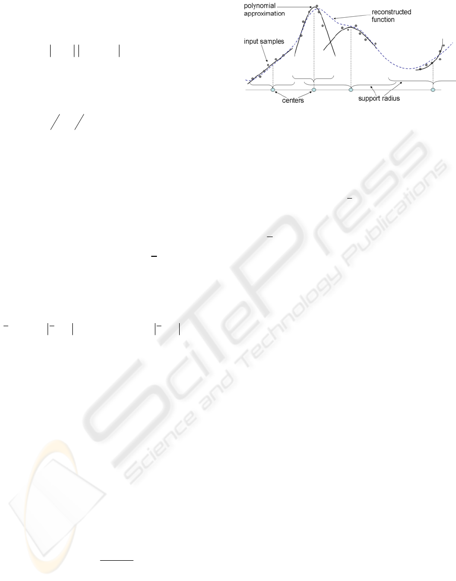
Figure 2: A diagram of the weighted least squares
approach to function representation. Each cente
r
constructs a low-degree polynomial approximation base
d
on samples in their neighborhood. These local
approximations are then combined to form a global
approximation.
AN INCREMENTAL WEIGHTED LEAST SQUARES APPROACH TO SURFACE LIGHTS FIELDS
87
approximation is computed from the samples in the
neighborhood list. As each center’s list gets larger,
the support radius is decreased, and samples are
discarded if they no longer fall within the
neighborhood. In our implementation, this involves
several user-defined parameters; we typically
decrease the radius by 25% if the number of samples
is more than 4 times the rank of the approximation.
3.3.2 Hierarchical Construction
The adaptive approach has the disadvantage that a
single sample can cause the recomputation of
numerous WLS coefficients, particularly in the
initial phases when the support radii are large. The
hierarchical approach avoids this computation by
subdividing the domain as a quadtree. Initially, the
representation consists of a single WLS center with
a large support radius. When a new image sample
arrives, the hierarchy is traversed until a leaf node is
reached. The sample is deposited at the leaf node
and the WLS is recalculated. If the number of
samples in a leaf node is larger than a pre-
determined threshold, the leaf node is split into four
children. Each child decreases its support radius and
recomputes its WLS coefficients. Note that a sample
can be a member of more than one leaf node, since
the support radii of the nodes can overlap. There are
several user-defined parameters; we have had good
results splitting the nodes if the number of samples
exceeds 4 times the rank of the approximation, and
decreasing the area of the neighborhood by half
(decreasing the radius by 1/√2).
3.4 Rendering
Weighted Least Squares conforms well to the
stream-processing model of modern graphics
hardware. Each surface patch is independent and is
calculated using a series of simple mathematical
operations (polynomial reconstruction and Partition
of Unity). More importantly, the local support of the
WLS centers means that reconstruction only requires
a few texture lookups in a small neighborhood.
After the centers and the WLS coefficients have
been computed (using either the adaptive or the
hierarchical technique), they are stored in a texture
map for each surface patch. The coefficients are laid
out in a grid pattern for fast access by the texture
hardware. The adaptive centers are typically
arranged in a grid pattern, but the hierarchical
pattern must be fully expanded before it is saved to
texture. This is done by copying down any leaf
nodes that are not fully expanded.
During rendering, the viewpoint is projected
onto the UV basis of the surface patch and used to
index into the coefficient texture. The samples from
the neighborhood around this element comprise the
set of overlapping WLS approximations. Texture
lookups are used to collect the neighboring centers
and their coefficients. These polynomial coefficients
are evaluated and weighted by their distance. The
weights are computed using the Partition of Unity,
which generates the final color for this surface patch.
Once the color at each patch has been
determined, we need a method to interpolate the
colors across the model to smoothly blend between
surface patches. One approach is to simply
interpolate the colors directly. However this
approach is incorrect, as it interpolates the values
after the Partition of Unity normalization step. This
generates artifacts similar to those encountered when
linearly interpolating normal vectors across a
triangle. The correct approach is to perform the
normalization after the interpolation. For our system,
we can accomplish this by interpolating the weights
and colors independently, and using a fragment
program to normalize the weights at every pixel.
4 IMPLEMENTATION
The data structure and camera capture are managed
on the CPU and function reconstruction and
rendering is handled by the GPU. In this section we
discuss how input images are converted into surface
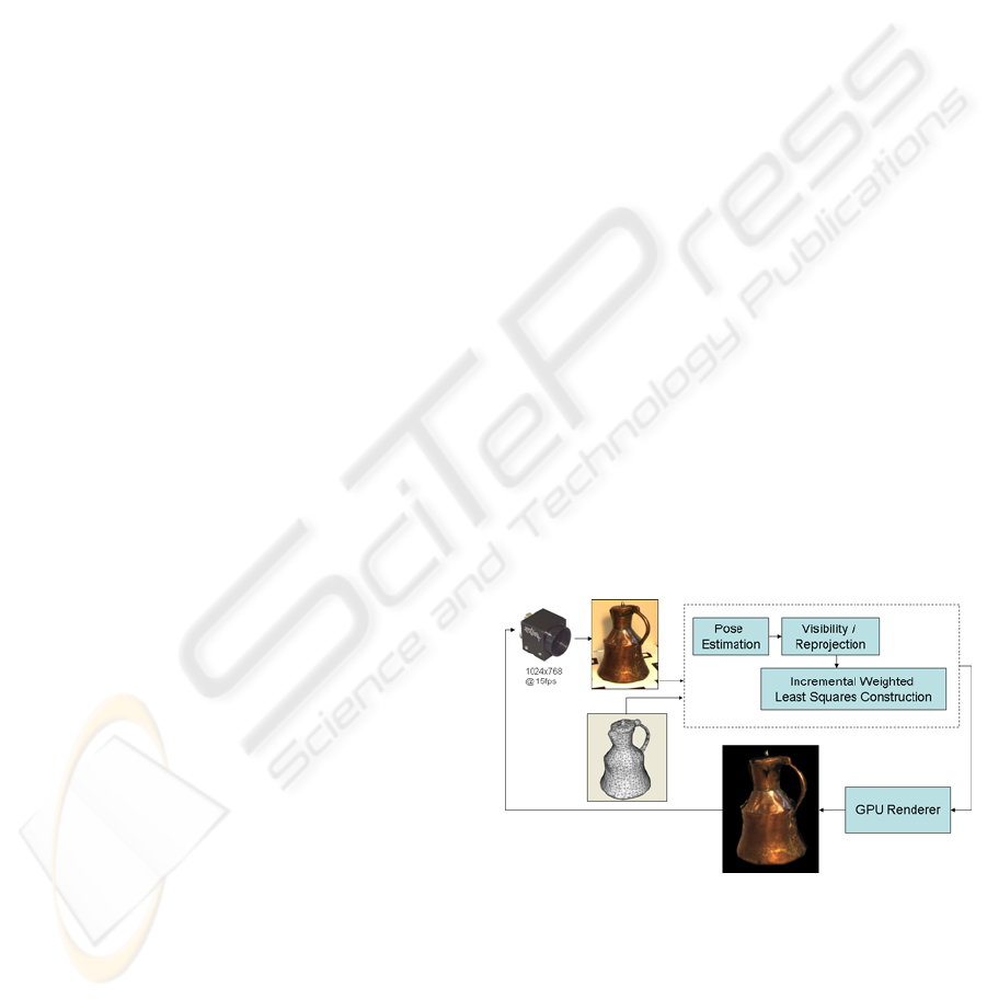
Figure 3: A diagram of the surface lightfield capture an
d
rendering system. Images are captured using a handhel
d
video camera, and passed to the system. Using the mesh
information, visibility is computed and the surface
locations are back-
p
rojected into the image. Each of these
samples are incorporated into the Incremental Weighte
d
Least Squares approximation, and sent to the card fo
r
rendering. The user can use this direct feedback to decide
where to move the video camera to capture more images.
GRAPP 2006 - COMPUTER GRAPHICS THEORY AND APPLICATIONS
88
patch samples, which involves camera capture, pose
estimation, and visibility computation. A diagram of
the system is shown in Figure 3.
In order to project the image samples onto the
geometry, the camera's position and orientation must
be known. Our system uses a tracked video camera
to capture images of the object. The camera was
calibrated with Bouguet’s Camera Calibration
Toolbox, and images are rectified using Intel`s Open
Source Computer Vision Library. To determine the
pose of the camera with respect to the object, a stage
was created with fiducials along the border. The 3D
positions of the fiducials are located in the camera's
coordinate system in real-time using the ARToolkit
Library. This library uses image segmentation,
corner extraction, and matching techniques for
tracking the fiducials. This system is similar to the
system presented in our earlier paper (Coombe,
2005).
Table 1: A description of the models and construction
methods used for timing data.
Once the camera pose has been estimated, the
visibility is computed by rendering the mesh from
the point of view of the camera. The depth buffer is
read back to the CPU, where it is compared against
the projected depth of each vertex. If the vertex
passes the depth test, it samples a color from the
projected position on the input image.
For rendering efficiency, the coefficient textures
are packed into a larger texture map. Each texture
stores the coefficients for one term of the
polynomial basis. For all of the examples in this
paper we use a 3-term polynomial basis. We found
that higher-order polynomial bases were susceptible
to over-fitting (Geman, 1992), which occurs when
the number of input samples is small enough that the
polynomial bases try to fit minor errors in the data,
rather than the overall shape. The consequence is
that reconstruction is very accurate at sample
positions, but oscillates wildly around the edges.
Using a lower-degree polynomial avoids this
problem.
The positions of the surface patches, which are
determined a priori, are represented as either
vertices or texels. For most of the models we use
vertices, and the renderer uses a vertex texture fetch
to associate surface patches with vertices.
4.1 Results
We have implemented this system on a 3.2 GHz
Intel Pentium processor with an Nvidia GeForce
7800. A graph of timing results from several
different models is shown in Figure 4, and the
parameters used for these timings are shown in
Table
1
. The rendering algorithm is compact, fast, and
efficient and can render all of the models in this
paper at over 200 frames per second. An image
Model # Vertices Construction # Centers
Bust A 31K Hierarchical 16
Heart A 4K Hierarchical 16
Pitcher A 29K Hierarchical 16
Bust B 14K Hierarchical 16
Bust C 14K Hierarchical 64
Heart B 4K Adaptive 16
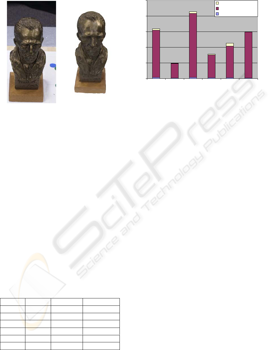
Figure 4: Timing results (in seconds per image) for the
IWLS construction. We measured three quantities; the time
to compute the visibility and reproject the vertices into the
image, the Least Squares fitting times, and the time to
transfer the computed results to the graphics card fo
r
rendering.
0
0.5
1
1.5
2
2.5
bust A heart A pitcher
A
bust B bust C heart B
Transfer
WLS
Visibility/Reprojection
Figure 5: A side-by-side comparison of the WLS
reconstruction with an input image that was not included
in the training set.
AN INCREMENTAL WEIGHTED LEAST SQUARES APPROACH TO SURFACE LIGHTS FIELDS
89
generated with our system is shown in Figure 1, and
a side-by-side comparison is shown in Figure 5.
The hierarchical construction method is much
faster than the adaptive construction method due to
the fact that the adaptive construction method can
potentially cause the recomputation of a number of
coefficients. For the 4K-vertex heart model, the
adaptive construction generated about 5.1 Least
Squares fitting computations per image, while the
hierarchical construction only generated about 1.7.
As this is the most time-consuming aspect of the
process, reducing the number of Least Squares fits is
important to achieve good performance. This
performance gain enables higher resolution
reconstruction; note that the bust model with 64
centers is only 1.4 times slower than the 16 center
version, even though it has 4 times as many
coefficients. However, the increased number of
coefficients is reflected in the data transfer time,
which is close to 4 times longer.
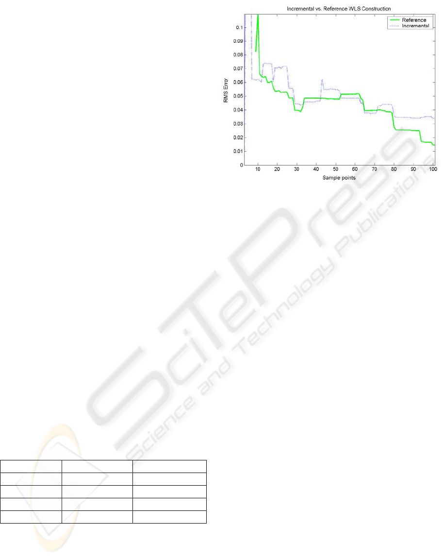
A potential issue with the hierarchical
construction is that it could introduce error. We
conducted an experiment to compare the quality of
the reconstruction with a reference batch process
which has global knowledge. The results are shown
in Figure 6.
We have tried several center placement
strategies; a uniform grid over projected hemisphere
directions, a uniform disk using Shirley’s concentric
mapping (Shirley, 1997), and jittered versions of
each. A comparison is shown in
Table 2. For most of
the models in this paper we use the grid method due
to its ease of implementation.
Table 2: RMS Error values from reconstructing a WLS
approximation while varying the center layout. The error
was computed with a training set of 64 images and an
evaluation set of 74 images. The disk is a slight
improvement in terms of error compared to the grid, and it
has a large benefit in terms of reducing the variability of
the error.
Layout Mean RMS Error StD RMS Error
Uniform Grid 0.0519 0.0086
Jittered Grid 0.0608 0.0148
Uniform Disk 0.0497 0.0045
Jittered Disk 0.0498 0.0036
5 CONCLUSION
We have introduced Incremental Weighted Least
Squares (IWLS), a fast, efficient, and incremental
algorithm for the representation and rendering of
surface light fields. IWLS can be used to render high
quality images of surfaces with complex reflectance
properties. The incremental construction is useful for
visualizing the representation as it is being captured,
which can guide the user to collect more images in
undersampled regions of the model and minimize
redundant capture of sufficiently sampled regions.
The rendering algorithm, which is implemented on
the GPU for real-time performance, provides
immediate feedback to the user.
5.1 Future Work
There are several improvements to our system that
we are interested in pursuing. Currently, the surface
patches are computed independently and do not
share information. This choice was made in order to
allow the algorithm to reconstruct as broad a class of
surfaces as possible. However, many surfaces have
slowly-varying reflectance properties which could
be exploited for computational gain. Each surface
patch could collect WLS coefficients from itself as
well as its neighbors. This would involve adjusting
the distance weighting to reflect the distance along
the surface of the model. We could also use an
approach similar to Zickler (Zickler, 2005) to share
reflectance values across a surface.
This system was designed to construct and
render surface light fields, which allow arbitrary
Figure 6: The reconstruction error of the hierarchical
construction versus a batch construction for a single surface
p
atch of the bust model. Each method used only the inpu
t
samples available, and the error was measured against the
full set of samples. The hierarchical algorithm is initially
superior to the batch algorithm, and continues to be simila
r
in error behavior while also being much faster to compute.
GRAPP 2006 - COMPUTER GRAPHICS THEORY AND APPLICATIONS
90

viewpoints but a fixed lighting. We are interested in
applying IWLS to the problem of reconstructing
arbitrary lighting, but from a static viewpoint. This
is similar to Polynomial Texture Mapping
(Malzbender, 2001), which used Least Squares
fitting and custom hardware to render images with
varying lighting.
Mathematically, the Weighted Least Squares
approach generalizes easily to multiple dimensions
by simply modifying the polynomial basis.
However, the substantial increase in data would
require re-thinking the construction and rendering
components of our system.
REFERENCES
Buehler, C., et al., 2001. Unstructured Lumigraph
Rendering. in SIGGRAPH 2001.
Carr, J.C., et al., 2001. Reconstruction and Representation
of 3D Objects with Radial Basis Functions. in
SIGGRAPH. 2001.
Chen, W.-C., et al., 2002. Light Field Mapping: Efficient
Representation and Hardware Rendering of Surface
Light Fields. in SIGGRAPH. 2002.
Coombe, G., et al., 2005. Online Construction of Surface
Light Fields. in Eurographics Symposium on
Rendering.
Debevec, P.E., C.J. Taylor, and J. Malik, 1996. Modeling
and Rendering Architecture from Photographs: A
Hybrid Geometry- and Image-Based Approach. in
SIGGRAPH. 1996.
Debevec, P.E., Y. Yu, and G.D. Borshukov, 1998.
Efficient View-Dependent Image-Based Rendering
with Projective Texture-Mapping. in Eurographics
Rendering Workshop. Vienna, Austria.
Furukawa, R., et al., 2002. Appearance based object
modeling using texture database: acquisition,
compression and rendering. Proceedings of the 13th
Eurographics workshop on Rendering. 257-266.
Gardner, A., et al. 2003. Linear Light Source
Reflectometry. in SIGGRAPH 2003.
Geman, S., E. Bienenstock, and R. Doursat, 1992. Neural
Networks and the Bias/Variance Dilemma. Neural
Computation,
4: p. 1-58.
Gortler, S.J. et al., 1996. The Lumigraph, in SIGGRAPH
96 Conference Proceedings, p. 43--54.
Hillesland, K., S. Molinov, and R. Grzeszczuk, 2003.
Nonlinear Optimization Framework for Image-Based
Modeling on Programmable Graphics Hardware. in
SIGGRAPH. 2003.
Lafortune, E.P.F., et al., 1997. Non-Linear Approximation
of Reflectance Functions. in SIGGRAPH 97.
Lensch, H.P.A. et al., 2001. Image-Based Reconstruction
of Spatially Varying Materials. in Eurographics
Workshop on Rendering.
Levoy, M. and P. Hanrahan, 1996. Light Field Rendering.
in SIGGRAPH. 96.
Malzbender, T., D. Gelb, and H. Wolters, 2001.
Polynomial Texture Maps. in SIGGRAPH 2001.
Matusik, W. et al., 2003. A Data-Driven Reflectance
Model. SIGGRAPH, 2003.
Matusik, W., M. Loper, and H. Pfister. 2004.
Progressively-Refined Reflectance Functions from
Natural Illumination. in Eurographics Symposium on
Rendering.
McAllister, D.K., A.A. Lastra, and W. Heidrich. 2002.
Efficient Rendering of Spatial Bi-directional
Reflectance Distribution Functions. in Graphics
Hardware 2002. Saarbruecken, Germany.
Moody, J.E. and C. Darken, 1989. Fast learning in
networks of locally-tuned processing units. Neural
Computation,
1: p. 281-294.
Mueller, G., et al. 2004. Acquisition, Synthesis and
Rendering of Bidirectional Texture Functions. in
Eurographics State of the Art Reports.
Nealen, A., 2004. An As-Short-As-Possible Introduction to
Least Squares, Weighted Least Squares and Moving
Least Squares Methods for Scattered Data
Approximation and Interpolation.
Nishino, K., Y. Sato, and K. Ikeuchi. 1999. Eigen-Texture
Method: Appearance Compression Based on 3D
Model in Proceedings of CVPR-99.
Ohtake, Y., et al. 2003. Multi-level Partition of Unity
Implicits. in SIGGRAPH 2003.
Ramamoorthi, R. and S. Marschner, 2002. Acquiring
Material Models by Inverse Rendering, in SIGGRAPH
2002 Course Materials.
Remington, K.A. and R. Pozo, 1996. NIST Sparse BLAS
User's Guide. National Institute of Standards and
Technology.
Schirmacher, H., W. Heidrich, and H.-P. Seidel, 1999.
Adaptive Acquisition of Lumigraphs from Synthetic
Scenes in Computer Graphics Forum.
Shepard, D., 1968. A two-dimensional interpolation
function for irregularly-spaced data. in Proceedings of
the 1968 23rd ACM national conference.
Shirley, P. and K. Chiu, 1997. A Low Distortion Map
Between Disk And Square. Journal of Graphics Tools,
2(3): p. 45-52.
Wendland, H., 1995. Piecewise polynomial,positive
definite and compactly supported radial basis
functions of minimal degree. Advances in
Computational Mathematics,
4: p. 389-396.
Wendland, H., 2005. Scattered Data Approximation.
Cambridge Monographs on Applied and
Computational Mathematics, ed. P.G. Ciarlet, et al.
Cambridge University Press.
Wood, D., et al. 2000. Surface Light Fields for 3D
Photography. in SIGGRAPH. 2000.
Yu, Y. et al., 1999. Inverse Global Illumination:
Recovering Reflectance Models of Real Scenes from
Photographs. in Siggraph 99. Los Angeles.
Zickler, T. et al., 2005. Reflectance Sharing: Image-based
Rendering from a Sparse Set of Images in
Eurographics Symposium on Rendering.
AN INCREMENTAL WEIGHTED LEAST SQUARES APPROACH TO SURFACE LIGHTS FIELDS
91
