
DIFFUSION BASED PHOTON MAPPING
Lars Schjøth & Ole Fogh Olsen
IT University of Copenhagen
Rued Langgaards Vej 7, 2300 Copenhagen S
Jon Sporring
University of Copenhagen
Universitetsparken 1, 2100 Copenhagen Ø
Keywords:
Ray-tracing, global illumination, photon mapping, caustics, density estimation, diffusion filtering.
Abstract:
Density estimation employed in multi-pass global illumination algorithms give cause to a trade-off problem
between bias and noise. The problem is seen most evident as blurring of strong illumination features. In
particular this blurring erodes fine structures and sharp lines prominent in caustics. To address this problem
we introduce a novel photon mapping algorithm based on nonlinear anisotropic diffusion. Our algorithm
adapts according to the structure of the photon map such that smoothing occurs along edges and structures and
not across. In this way we preserve the important illumination features, while eliminating noise. We call our
method diffusion based photon mapping.
1 INTRODUCTION
Particle tracing is an important concept in global illu-
mination. Particle tracing algorithms usually employ
two passes. A first pass in which particles represent-
ing light are emitted from light sources and reflected
around a scene, and a second pass which generates an
image of the scene using the light transport informa-
tion from the first pass. Common to all algorithms
using particle tracing is that they trace light from the
light sources. This generates information about lights
propagation through the scene. In turn this informa-
tion is used to reconstruct the illumination seen in the
generated image. The advantage of particle tracing al-
gorithms is that they effectively simulate all possible
light paths. In particular they can simulate lighting
phenomena such as color bleeding and caustics.
However, particle tracing algorithms are faced with
a severe problem. In the particle tracing pass, parti-
cles are stochastically emitted from the light sources
and furthermore often stochastically traced through
possible light paths. This procedure induces noise,
which has to be coped with in the reconstruction of
the scene illumination. Unfortunately, the technique
used to reduce noise also introduce a systematic er-
ror (bias) seen as a blurring of the reconstructed illu-
mination. This is not necessarily a bad effect when
concerned with slowly changing illumination, but it
becomes an important problem when the illumination
intensity changes quickly such as when concerned
with caustics and shadows. This is a density estima-
tion problem well-known in classical statistics.
In this paper we develop an algorithm which re-
duces noise and in addition preserve strong illumina-
tion features such as those seen in caustics. We have
chosen to implement it in photon mapping. Photon
mapping is a popular particle tracing algorithm devel-
oped by Henrik Wann Jensen (Jensen, 1996).
Our algorithm is inspired by a filtering method
called nonlinear anisotropic diffusion. Nonlinear
anisotropic diffusion is a popular method commonly
used in image processing. It has the property of
smoothing along edges in an image instead of across
edges. Thus it preserves structures in an images while
smoothing out noise. We call this novel algorithm dif-
fusion based photon mapping.
Figure 1 illustrates two renderings; one using reg-
ular photon mapping and the other using diffusion
based photon mapping. The images shows how dif-
fusion based photon mapping reproduces caustics in
higher detail than regular photon mapping.
Despite the fact that diffusion filtering is almost ex-
clusively employed to process images, our method is
not a post-processing step applied to photon mapping
generated images. In diffusion based photon mapping
we have adapted diffusion filtering in order to employ
it on densities of photons during the illumination re-
construction.
168
Schjøth L., Fogh Olsen O. and Sporring J. (2006).
DIFFUSION BASED PHOTON MAPPING.
In Proceedings of the First International Conference on Computer Graphics Theory and Applications, pages 168-175
DOI: 10.5220/0001358101680175
Copyright
c
SciTePress
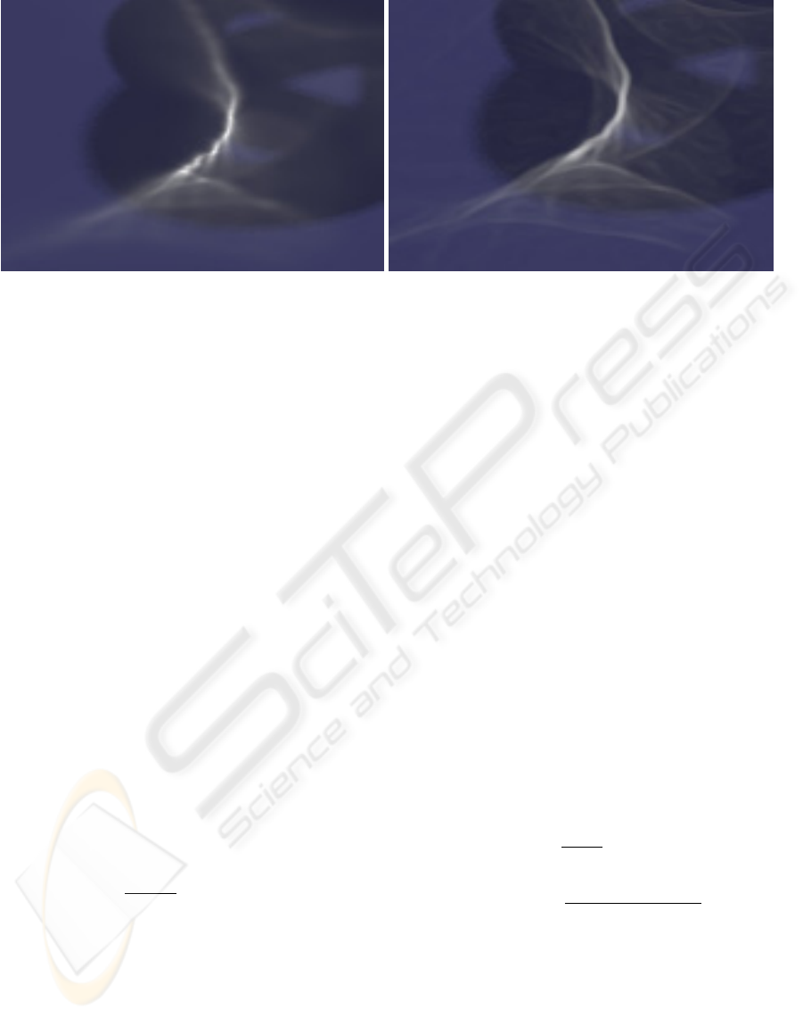
Figure 1: [a b] Rendering of caustics created by a glass torus knot. Region zoom from Figure 3. a) Using regular photon
mapping with cone filtering, b) using diffusion based photon mapping.
2 DENSITY ESTIMATION IN
PHOTON MAPPING
In photon mapping indirect illumination is recon-
struction through a series of queries to the photon
maps. A photon map is a collection of photons cre-
ated during a particle tracing phase in which photons
are reflected around a scene using Monte Carlo ray
tracing. Each query is used to estimate the reflected
radiance at a surface point as the result of a local pho-
ton density estimate. This estimate is called the radi-
ance estimate.
2.1 The Radiance Estimate
In his book (Jensen, 2001) Jensen derives an equa-
tion which approximates the reflected radiance using
the photon map. This is done by letting the incoming
radiance, L
i
, at a point be represented by the incom-
ing flux and letting the incoming flux at that point be
approximated using the point’s k nearest photons. In
this way the equation for the reflected radiance be-
comes
L
r
(x,ω) ≈
L
r
(x,ω)=
1
πr(x)
2
k
i=1
f
r
(x,ω
i
,ω)Φ
i
.
(1)
The equation sums over the k photons nearest the
point x. Φ
i
is the flux represented by the i’th photon,
f
r
is the bidirectional reflectance distribution func-
tion (abbreviated BRDF), and r(x) is the radius of
a sphere encompassing the k nearest photons, where
πr(x)
2
is the sphere’s cross-sectional area through its
center. The radius dependens on x, as the its value is
determined by the photon density in the proximity of
x. In density estimation r(x) is the called the band-
width, smoothing parameter or the windows width,
we will use the terms bandwidth and support radius
in this article.
The support radius is important because its size
controls the trade-off between variance and bias. A
small radius gives a limited support of photons in the
estimate; it reduces the bias but increases the variance
of the estimate. Inversely, estimating the radiance us-
ing a large radius results in an increase in bias and a
decrease in variance.
Using a k’th nearest neighbor search to decide the
support radius, Jensen helps limit bias and variance
in the estimate by smoothing more where the photon
density is sparse and less where the photon density is
dense.
The radiance estimate in Equation 1 is simple in-
sofar it weights each photon in the estimate equally.
Jensen refined the radiance estimate in (Jensen, 1996)
such that filtering was used to weight each photon ac-
cording to its distance to the point of estimation.
It is possible to reformulate the radiance estimate
to a general form such that it can be used with dif-
ferent filtering techniques. We formulate this general
radiance estimate as
L
r
(x,ω)=
1
r(x)
2
·
·
k
i=1
K
(x − x
i
)
T
(x − x
i
)
r(x)
2
·
· f
r
(x,ω
i
,ω)Φ
i
,
(2)
where x
i
is the position of the i’th photon and K(y)
is a function that weights the photons according to
their distance from x. This function should be sym-
metric around x and it should be normalized such that
it integrates to unity within the distance r(x) to x.In
density estimation K(y) is known as the kernel func-
tion. Usually, the kernel function decreases monoton-
ically, weighting photons near x higher than those far-
DIFFUSION BASED PHOTON MAPPING
169

ther away. In this way the kernel function reduce bias
where the change in density is significant.
In his PhD thesis (Jensen, 1996) Jensen presents
the cone filter. This filter is used to reduce bias, such
that edges and structure in the illumination are less
blurred. As a kernel in the general radiance estimate
the cone filter has the following form
K(y)=
K(y)=
1−
√
|y|
k
(1−
2
3k
)π
if
|y| < 1,
0 otherwise,
(3)
where k ≥ 1 is a constant which controls the steep-
ness of the filter slope.
Another useful kernel is the Epanechnikov kernel.
The Epanechnikov kernel is known from statistics for
its bias reducing properties and it is furthermore pop-
ular because it is computationally inexpensive. In
computer graphics, Walter has employed it with good
results in (Walter, 1998). In 2D the Epanechnikov ker-
nel is given by
K(y)=
2
π
(1 − y)ify < 1,
0 otherwise.
(4)
In this paper we use the Epanechnikov kernel to ex-
amine our proposed method.
2.2 Bias Reduction
Bias reduction is a well examined subject, when con-
cerned with density estimation both within the field of
statistics and the field of computer graphics. Besides
filtering, numerous methods addressing the issue has
been presented.
The first method for reducing bias in photon map-
ping was suggested by Jensen (Jensen and Chris-
tensen, 1995). The method is called differential
checking and it reduces bias by making sure that the
support radius of the radiance estimate does not cross
boundaries of distinct lighting features. This is done
by expanding the support radius ensuring that the es-
timate does not increase or decrease, when more pho-
tons are included in the estimate.
Myszkowsky et al. (Myszkowski, 1997) suggested
to solve the problem in much the same way as Jensen
did with differential checking, however, they made
the method easier to control and more robust with re-
spect to noise. Myszkowsky et al. increase the sup-
port radius iteratively estimating the radiance in each
step. If new estimates differ more from previous than
what can be contributed variance, the iteration stops
as the difference is then assumed to be caused by bias.
More recently Schregle (Schregle, 2003) followed-
up their work using the same strategy but optimizing
speed and usability. Speed is optimized by using a
binary search for the optimal support radius. This
search starts in a range between a maximum and a
minimum user-defined support radius. The range is
split up, and the candidate, whose error is most likely
to be caused by variance and not bias, is searched.
Shirley et al. (Shirley et al., 1995) introduced an
algorithm for estimating global illumination. Like
photon mapping this algorithm uses density estima-
tion to approximate the illumination from particles
generated during a Monte Carlo-based particle trac-
ing step. However, unlike photon mapping the algo-
rithm is gemoetry-dependent - the illumination is tied
to the geometry. They called the algorithm the density
estimation framework and they refined it in a series of
papers.
The first edition of their framework did not try to
control bias. In (Walter et al., 1997) they extended
the framework to handle bias near polygonal bound-
aries. This was done by converting the density estima-
tion problem into one of regression. In this way they
could use common regression techniques
1
to elimi-
nate boundary bias.
Later Walter in his PhD thesis (Walter, 1998), re-
duced bias by controlling the support radius of the
estimate using statistics to recognize noise from bias.
Benefiting from the field of human perception he used
a measure for controlling the support radius such that
noise in the estimate was imperceptible to the human
eye.
Walter recognized that if bias was to be signifi-
cantly reduced, using his method, perceptual noise
had to be accepted in the vicinity of prominent edges
and other strong lighting features. This is a common
problem which also affects differential checking and
both Schregle’s and Myszkowsky’s method. Hence,
in the proximity of strong features such as the edges
of a caustic the support radius stops expanding and the
foundation on which the estimate is made is supported
by few photons. This means that when estimates are
made close to edges the support is limited and noise
may occur.
In diffusion based photon mapping we employ
the concept of nonlinear anisotropic diffusion in the
radiance estimate of photon mapping. Nonlinear
anisotropic diffusion is a well examined and popular
technique within the field of image analysis. It is a fil-
tering technique that adapts its smoothing according
to the image structure. This means that it smoothes
along edges and not across. It is known to be robust
and effective (Weickert, 1998). To our knowledge the
technique has not been employed in connection with
photon mapping.
In contrast to Myszkowsky, Schregle and Walter’s
approach our method will smooth along edges and
structures, it follows that its support will not be lim-
ited in the proximity of these.
1
Specifically they used locally-weighted polynomial
least-squares regression to eliminate boundary bias.
GRAPP 2006 - COMPUTER GRAPHICS THEORY AND APPLICATIONS
170
3 ANISOTROPIC FILTERING IN
PHOTON MAPPING
To be able to use anisotropic filtering in photon map-
ping, we in some way have to be able describe the
structure of the photon map, to get some guidance as
how to adapt the filtering. It follows that it is neces-
sary to modify the radiance estimate such that the ker-
nel adapts according to the structure description and
that we, furthermore, need to normalize this modified
radiance estimate in order to preserve energy when
the kernel changes shape.
3.1 Structure Description
The gradient of the illumination function denotes
the orientation in which the illumination intensity
changes and therefore describes the first order struc-
ture of the illumination. This information will be used
to steer the filtering.
As the illumination function is estimated in the ra-
diance estimate, the differentiated radiance estimate
approximates the gradient of the photon map.
To differentiate the radiance estimate we combine
the generalized radiance estimate from Equation 2,
with a suitable kernel function. Furthermore, it is con-
venient to simplify the radiance estimate by assuming
that all surfaces hit by photons are ideal diffuse re-
flectors. This means that the BRDF, f
r
, is constant
regardless of the incoming and outgoing direction of
light. In this way the BRDF does not need to be dif-
ferentiated as it does not depend on the position, x,
which is the variable in respect to which we differen-
tiate.
This of course is a radical assumption as photons
can be affected much by the type of surfaces they en-
counter. However, photons are only stored on diffuse
surfaces, so the surfaces involved in the radiance es-
timate are most likely diffuse and need therefore not
differ much from an ideal diffuse surface. Further-
more if we were to differentiate the BRDF then our al-
gorithm would not be able to handle arbitrary BRDFs
as we would have to know the BRDF in order to do so.
In effect we would not retain the beneficial qualities
of photon mapping. Another solution would of course
be to do reverse engineering, to numerically estimate
the BRDF in question, however, this approach is both
cumbersome and computationally expensive.
Additionally, we have to make a constraint on the
generalized radiance estimate. The estimate should
use a fixed support radius for r(x) such that the radius
is independent of x. Though this effectively reduces
the radiance estimate to a common multivariate kernel
estimator - rather than a k’th nearest neighbor estima-
tor - this is not a severe constraint. The advantage of
the k’th nearest neighbor search is its ability to reduce
bias. This ability is important in the radiance estimate,
however, when estimating the gradient, smoothing is
an advantage as the gradient is perceptible to noise.
Combining a simplified version of the generalized
radiance estimate with the two-dimensional Epanech-
nikov kernel we get
L
r
(x,ω)=
2f
r
πr
2
k
i=1
1 −
(x − x
i
)
T
(x − x
i
)
r
2
Φ
i
,
(5)
This equation can be differentiated giving us the gra-
dient function of the estimated illumination function.
Differentiating Equation 5 with respect to the j’th
component of x gives the partial derivative
∂
L
r
(x,ω)
∂x
j
=
4f
r
πr
2
k
i=1
−
x
j
− x
ij
r
2
Φ
i
. (6)
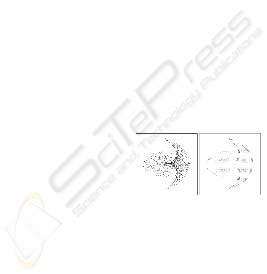
As seen from Figure 2, the gradient of the photon map
is a plausible structure descriptor. Figure 2a is a distri-
bution of photons and Figure 2b is a gradient field of
the distribution. The gradient vectors are calculated
using the photons nearest the center of each quadrant
in the grid of the field. The gradient vectors along the
edges of the distribution are those with greatest mag-
nitude and the vectors are as expected perpendicular
to edges and structures.
Figure 2: [a b] a) Cardioid shaped photon distribution cre-
ated by light reflection within a metal ring, b) gradient field
of the photon distribution in a).
We denote the gradient of the photon map ∇M,
where M is the photon map.
A more advanced way is to describe the first order
structure is with the structure tensor. The structure
tensor was introduced to diffusion filtering by Weick-
ert (Weickert, 1995). The advantage of the structure
tensor is that even though it does not contain more in-
formation than the gradient descriptor, it is, unlike the
gradient, possible to smooth it without losing impor-
tant structure information. Being able to smooth the
structure descriptor makes the orientation information
less perceptible to noise.
DIFFUSION BASED PHOTON MAPPING
171

The structure tensor is the tensor product of the gra-
dient. In three dimensions it is given by
∇M ⊗∇M =
⎛
⎝
M
2
x
M
x
M
y
M
x
M
z
M
x
M
y
M
2
y
M
y
M
z
M
x
M
z
M
y
M
z
M
2
z
⎞
⎠
.
(7)
In diffusion based photon mapping we use the struc-
ture tensor to describe the structure of the photon
map.
3.2 Diffusion Tensor
In diffusion filtering the filtering is controlled by a
symmetric positive semidefinite matrix called the dif-
fusion tensor (Weickert, 1998). This matrix can be
constructed using information derived from a struc-
ture descriptor. One possible construction is for edge
enhancing which will be apply in this paper to pre-
serve the finer structures of the illumination.
For edge enhancing, smoothing should occur paral-
lel to the edges not across them. The orientation of the
local edge structure is derived from the structure ten-
sor. The primary eigenvector of the structure tensor
is simply the gradient which is perpendicular to the
local edge orientation. The direction parallel to edges
can be calculated as the cross-product of the surface
normal and the vector representing the direction par-
allel to the structure. This will be the main direction
of diffusion.
The eigenvectors and eigenvalues of the diffusion
tensor describe respectively the main directions of dif-
fusion and the amount of diffusion in the correspond-
ing direction. Hence by constructing the diffusion
tensor from the primary eigenvector of the structure
tensor diffusion can be steered to enhance the edges.
The gradient of the illumination function (derived
from the structure tensor) is only in the tangent plane
to the surface if the surface is locally flat. Since the
photon energy should stay on the surface we must in-
sure that the main diffusion direction is the tangent
plane.
Consequently, the diffusion directions are con-
structed in the following way.
The primary eigenvector of the structure tensor is
projected to the plane perpendicular to the surface
normal. This is our second diffusion direction
X
2
.
The third diffusion direction is the surface normal
X
3
and the primary diffusion direction is the cross prod-
uct of the second and third diffusion direction
X
1
. All
vectors should be normalized.
The diffusion tensor is constructed as
D = X diag(λ
1
,λ
2
,λ
3
) X
T
,
(8)
where X is [
X
1
X
2
X
3
] and diag(·) is the diagonal ma-
trix containing the eigenvalues of D along the diago-
nal.
It remains to determine the amount of diffusion.
That is the eigenvalues, λ:
λ
1
=1,
λ
2
=
1
1+
µ
1
K
1+α
,α>0,
λ
3
=0.1,
(9)
where the secondary eigenvalue, λ
2
, is estimated us-
ing a function called the diffusivity function, intro-
duced to diffusion filtering by Perona and Mallik (Per-
ona and Malik, 1990). The diffusivity coefficient, K,
decides when the function starts to monotonically de-
crease and α the steepness of the decline. In practice
what it means is, that K is the threshold deciding what
value of the primary eigenvalue of the structure ten-
sor, µ
1
, is considered an edge and what is considered
noise, and α controls the smoothness of transition.
We suggest that the tertiary eigenvalue, λ
3
should
be set to 0.1. The reason why the tertiary vector
should have such a low eigenvalue is that it limits cer-
tain forms of bias. It is comparable to using a disc
instead of a sphere to collect photons; a techniques to
reduce bias in corners (Jensen, 2001).
We have now constructed a diffusion tensor which
favors diffusion parallel to structures while limiting
diffusion perpendicular to structures. We will utilize
this tensor such that it controls the filtering of the pho-
ton map.
3.3 The Diffusion Based Radiance
Estimate
The next step is to use the diffusion tensor to shape the
kernel of the radiance estimate such that it smoothes
along structures and edges and not across. To do this
we have to shape our kernel in some way.
If we take a look at the multivariate kernel density
estimator on which the radiance estimate is based,
f(x)=
1
nh
d
n
i=1
K
(x − x
i
)
T
(x − x
i
)
h
2
,
(10)
it is important to note that the kernel is uniform inso-
far that only a single parameter, h is used. Data points,
x
i
, are scaled equally according to the bandwidth, h,
and their distance to the center, x. Smoothing occurs
equally in all directions.
Now considering a simple two dimensional normal
distribution:
f(x)=
1
2πσ
1
σ
2
exp
−
(x
1
− µ
1
)
2
√
2σ
1
−
(x
2
− µ
2
)
2
√
2σ
2
,
(11)
GRAPP 2006 - COMPUTER GRAPHICS THEORY AND APPLICATIONS
172

where σ
1
and σ
2
are the standard deviations with re-
spect to the axes and µ is the center of the distribution.
Here we have a Gaussian kernel whose shape is spec-
ified by the two parameters for the standard deviation.
Unfortunately, this equation only gives control in two
directions.
However, generalizing the equation to d dimen-
sions, we can use an inversed d×d covariance matrix,
Σ
−1
, to shape the normal distribution:
f(x)=
1
(2π)
d/2
√
det Σ
·
· exp
−
(x − µ)
T
Σ
−1
(x − µ)
2
.
(12)
In two dimensions using a diagonal covariance matrix
with the variance values in the diagonal this equation
is exactly the same as Equation 11. However, using
a matrix we are not limited to control the shape of
the Gaussian in only two direction. If we for exam-
ple had shaped our Gaussian kernel to form an ellipse,
we could rotate this kernel by rotating the covariance
matrix. The equation will remain normalized as the
determinant of a matrix is rotational invariant. So the
shape of normal distribution in Equation 12 is con-
trolled by the covariance matrix.
We can use Equation 12 to extend the generalized
radiance estimate from Equation 2. To generalize the
shape adapting properties we use the Mahalanobis
distance from Equation 12 to shape the kernel. The
Mahalanobis distance is a statistical distance. It is
given by:
d(x, y)=(x − y)
T
Σ
−1
(x − y). (13)
As the shape of the kernel should be controlled by the
diffusion tensor we use the tensor in place of the co-
variance matrix. We can reformulate the generalized
radiance estimate as:
L
r
(x,ω)=
1
r
2
√
det D
·
·
k
i=1
K
(x − x
i
)
T
D
−1
(x − x
i
)
r
2
·
· f
r
(x,ω
i
,ω)Φ
i
.
(14)
We now have a general diffusion based radiance esti-
mate, which filters the photon map adapting the shape
of the kernel according to the diffusion tensor. Or to
be even more general we have a radiance estimator
which estimates the illumination function taking into
consideration the structure of the photon map, such
that edges and structures are preserved.
3.4 Implementation
Diffusion based photon mapping can be implemented
in different ways depending on which structure de-
scriptor is used, however, we propose to use the struc-
ture tensor and for this reason we need to estimate it
or have it available during the radiance estimate in or-
der to construct the diffusion tensor.
We do this using a preprocessing step that approx-
imates the gradient of the photon map. The pre-
processing step occurs between the photon tracing
pass and the rendering pass. To approximate the gra-
dient we sample it at all photon positions. The advan-
tage of this procedure is that we can store the local
gradient along with the photon and in this way does
not need a separate gradient map. Additionally, we
know the sampling positions to be located on a sur-
face, as photons are only stored in connection with a
surface. This is useful as the gradient is only relevant
at surface positions.
During the radiance estimate we calculate the struc-
ture tensors at the photon positions near x. In this
way we can estimate the local structure tensor as the
weighted average of the surrounding structure ten-
sors. Smoothing the structure tensor reduces noise
and furthermore gives a broader foundation from
which to steer the filtering after.
Having calculated the local structure tensor we
construct the diffusion tensor as described in the for-
mer section. This then is used in the general diffusion
based radiance estimate together with a suitable ker-
nel.
For a more through examination of diffusion based
photon mapping refer to (Schjøth, 2005).
4 RESULTS
Figure 3 is a rendering of a scene consists of a simple
glass torus knot positioned over a plane in space. A
spherical light source above the torus knot creates the
caustic on the plane.
Figure 3a illustrates the scene visualized employ-
ing the k’th nearest neighbor estimate in conjunction
with the cone kernel whereas Figure 3b is visualized
using diffusion based photon mapping.
The difference in the two images is seen in the
caustics. The structure of the caustic in Figure 3b
is much more detailed than the caustic in Figure 3a.
Fine patterns are visible in the caustic in the image
estimate using the diffusion based radiance estimate
that are not visible in the image estimated using the
cone kernel.
To further test diffusion based photon mapping we
have constructed a photon distribution. The con-
structed distribution is rather simple yet it contains
both edges and ridges and circular and rectangular
shapes.
DIFFUSION BASED PHOTON MAPPING
173
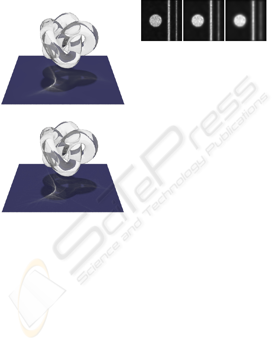
Figure 3: [
a
b
] Rendering of a glass torus positioned above
a plane using a) regular photon mapping and b) diffusion
based photon mapping.
4.1 The Cone Kernel
We first test Jensen’s cone kernel on the constructed
distribution. This is done by first combining the cone
kernel from Equation 3, with the general radiance es-
timate from Equation 2. We then estimate the radi-
ance of the constructed photon distribution a number
of times, iteratively expanding the support radius, al-
lowing an increasing amount of photons in each esti-
mation. This is done until the result contains an ac-
ceptable low noise level. The result of this procedure
is illustrated in Figure 4. It is seen from the illustra-
tion that the noise level decreases slowly with respect
to the number of photons per estimate. Bias is visi-
ble as a clearly identifiable blurring of shape edges.
In addition boundary bias is seen along the bound-
aries of the images. It should be clear that the bias
increases as the noise is reduced. This phenomenon
Figure 4: [a b c] A visualization of a constructed distrib-
ution estimated using the cone kernel. a) estimated using
the 200 nearest photons, b) estimated using the 400 nearest
photons and, c) estimated using the 800 nearest photons.
is directly related to the bias vs. variance trade-off ac-
counted earlier. Another thing to notice is how the
thin line losses intensity as the number of photons per
estimate is increased. This happens because the en-
ergy of the line is spread out over a larger area as the
smoothing increase.
4.2 The Diffusion Based Radiance
Estimate
To test the applicability of the structure tensor as
structure descriptor, we use the diffusion based radi-
ance estimate together with the Epanechnikov kernel.
In contrast to the cone kernel radiance estimate we
will not us the k nearest neighbor method to reduce
bias, instead we will use a fixed support radius letting
the shape adaption reduce bias.
We first set the support radius low, and then we it-
eratively increase the support radius until the noise
level is acceptable. This is done using a large value of
the diffusivity coefficient K from Equation 9. In this
way the kernel will stay uniform and will not adapt
according to structure. Estimating the radiance with a
uniform Epanechnikov kernel using different support
radii we find a support radius which reduces noise to
an acceptable level.
Using this support radius we test the diffusion
based radiance estimate by iteratively decreasing the
value of the diffusivity coefficient such that the ker-
nel starts to adapt its shape according to the structure
described by the structure tensor. The result of this
procedure is illustrated in Figure 5. From the results
of the diffusion based radiance estimate we see that
edges are enhanced as the diffusivity coefficient is de-
creasing.
4.3 Summary of the Visual Results
We summarily compare the best results of the two ra-
diance estimation methods. The results were chosen
in the attempt to find the estimates with least noise
and least bias. Figure 6 depicts the estimates. From
GRAPP 2006 - COMPUTER GRAPHICS THEORY AND APPLICATIONS
174
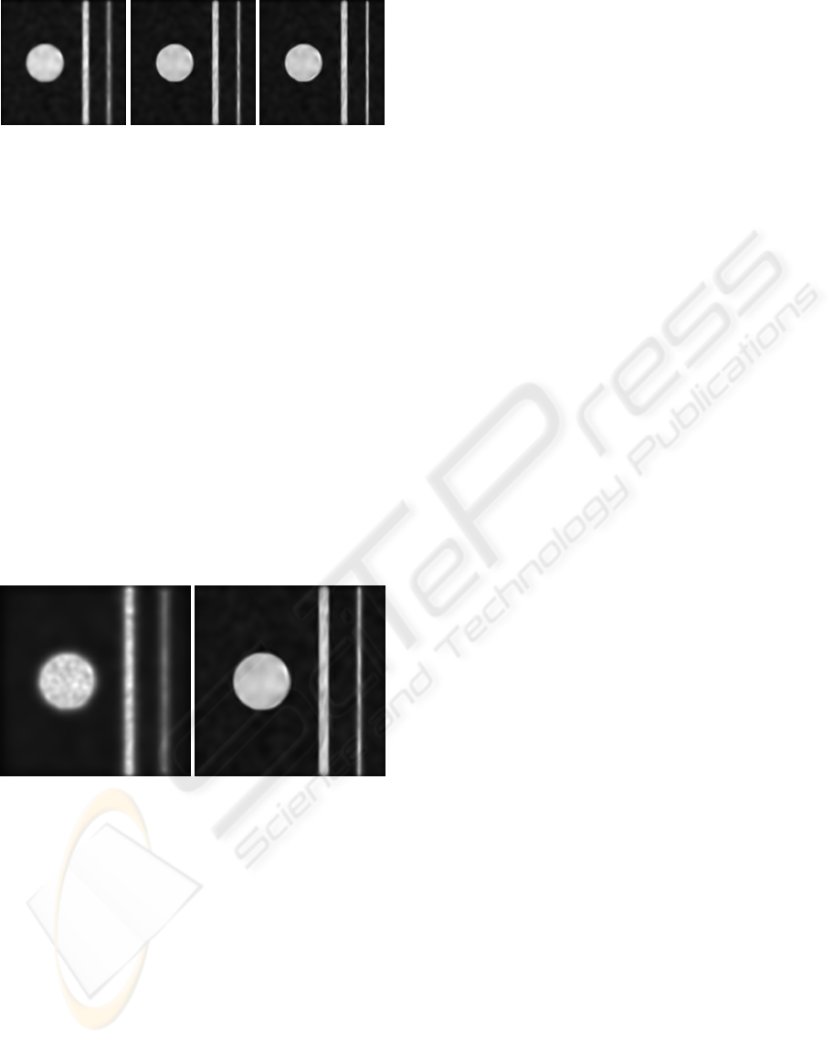
Figure 5: [a b c] A visualization of a constructed distrib-
ution estimated using diffusion based photon mapping. a)
estimated using K=0.4, b) estimated using K=0.2 and, c)
estimated using K=0.1.
the chosen results we see that the diffusion based ra-
diance estimates reduces bias markedly better than
the common k’th nearest neighbor radiance estimate.
However, background noise is less pronounced in the
common radiance estimate.
Another thing to notice is the thinnest line in the
constructed distribution. We know that this line has
photon distribution as dense as the two other shapes
in the distribution. For this reason the thin line should
be just as intense as the other shapes. However, as
estimates are smoothed using a higher support radius
and more photons per estimate, the energy is spread
out. Comparing the three results it is seen that the
structure based radiance estimate is most successful in
preserving the energy of the thin line as it has almost
the same intensity as the other shapes.
Figure 6: [a b] A visualization of a constructed distribu-
tion estimated using different radiance estimation methods.
a) estimated using a uniform cone kernel with 400 photons
per estimate and b) estimated using a gradient based shape
adapting Gaussian radiance estimate with a diffusivity co-
efficient of K = 0.2.
Finally, it should be mentioned that it has not been
our objective to test the computationally performance
diffusion based photon mapping. Despite this we will
say a few things about the running time. Considering
the estimates of the constructed distribution. The im-
age in Figure 6a was estimated using the cone kernel
and 400 photons per estimate. It was computed in 45
seconds. In comparison the computation time for the
tensor based radiance estimate, producing Figure 6b,
was 1 minute and 3 seconds from which 12 seconds
was used estimating the gradient map.
5 CONCLUSION
In this paper we have proposed a novel method for
enhancing edges and structures of caustics in parti-
cle tracing algorithms. Our method is called diffusion
based photon mapping.
The method is based on nonlinear anisotropic dif-
fusion which is a filtering algorithm known from im-
age processing. We have implemented it in photon
mapping and we have shown that our algorithm is
markedly better than regular photon mapping when
simulating caustics. Specifically, does diffusion based
photon mapping preserve edges and other prominent
features of the illumination where as regular photon
mapping blur these features.
REFERENCES
Jensen, H. W. (1996). The Photon Map in Global Illumi-
nation. PhD thesis, Technical University of Denmark,
Lyngby.
Jensen, H. W. (2001). Realistic image synthesis using pho-
ton mapping. A. K. Peters, Ltd., Natick, MA, USA.
Jensen, H. W. and Christensen, N. J. (1995). Photon maps in
bidirectional monte carlo ray tracing of complex ob-
jects. Computers & Graphics, 19(2):215–224.
Myszkowski, K. (1997). Lighting reconstruction using fast
and adaptive density estimation techniques. In Pro-
ceedings of the Eurographics Workshop on Render-
ing Techniques ’97, pages 251–262, London, UK.
Springer-Verlag.
Perona, P. and Malik, J. (1990). Scale-space and edge de-
tection using anisotropic diffusion. IEEE Transactions
on Pattern Analysis and Machine Intelligence, PAMI-
12(7):629–639.
Schjøth, L. (2005). Diffusion based photon mapping. Tech-
nical report, IT University of Copenhagen, Copen-
hagen, Denmark.
Schregle, R. (2003). Bias compensation for photon maps.
Computer Graphics Forum, 22(4):729–742.
Shirley, P., Wade, B., Hubbard, P. M., Zareski, D., Wal-
ter, B., and Greenberg, D. P. (1995). Global illumi-
nation via density-estimation. Rendering Techniques
’95, pages 219–230.
Walter, B. (1998). Density estimation techniques for global
illumination. PhD thesis, Cornell University.
Walter, B., Hubbard, P. M., Shirley, P., and Greenberg, D. P.
(1997). Global illumination using local linear density
estimation. ACM Trans. Graph., 16(3):217–259.
Weickert, J. (1995). Multiscale texture enhancement. Lec-
ture Notes in Computer Science, 970:230–237.
Weickert, J. (1998). Anisotropic Diffusion in Image
Processing. B. G. Teubner, Stuttgart, Germany.
DIFFUSION BASED PHOTON MAPPING
175
