TERRAIN SYNTHESIS BY-EXAMPLE

John Brosz, Faramarz F. Samavati and Mario Costa Sousa

University of Calgary

2500 University Drive NW, Calgary, Canada

Keywords:

Terrain synthesis, modeling, multi-resolution analysis, multi-fractals.

Abstract:

Synthesizing terrain or adding detail to terrains manually is a long and tedious process. With procedural

synthesis methods this process is faster but more difﬁcult to control. This paper presents a new technique of

terrain synthesis that uses an existing terrain to synthesize new terrain. To do this we use multi-resolution

analysis to extract the high-resolution details from existing models and apply them to increase the resolution

of terrain. Our synthesized terrains are more heterogeneous than procedural results, are superior to terrains

created by texture transfer, and retain the large-scale characteristics of the original terrain.

1 INTRODUCTION

Terrain synthesis is the process of creating the artiﬁ-

cial terrains used in games, movies, and simulations.

Artiﬁcial terrains are necessary whenever terrain in-

formation is not available, lacks resolution and detail,

or must meet speciﬁc feature criteria. Creating arti-

ﬁcial terrain is not easy as large, high-resolution ter-

rains often involve millions of data points.

There are two major applications of terrain synthe-

sis. The ﬁrst is in creating a synthetic terrain guided

by a user who provides a rough outline of the desired

characteristics. In this case the goal is to retain the

attributes of the given outline, while adding realistic

features to ﬁll out the terrain. The second application

is in increasing the resolution of an existing terrain for

close-up viewing. Although any type of surface in-

terpolation can increase resolution, it will also make

the terrain look overly smooth. Extra information in

the form of deviation from the smooth surface is nec-

essary to make the terrain interesting and realistic.

Terrains synthesized for both applications should ap-

pear visually realistic, meet desired topology require-

ments, and be inexpensive in terms of modeling time

(Roettger and Frick, 2002).

Presently in commercial systems like Bryce

(Bryce, 2005) and Terragen (McLusky, 2005), arti-

ﬁcial terrains are created through a mixture of pro-

cedural methods and user painting of height ﬁelds

(Roettger and Frick, 2002). The procedural methods,

usually based on fractal subdivision, are controlled by

user speciﬁed parameters. These methods have major

shortcomings in that they lack erosion features and

create homogeneous terrains. To compensate for this,

erosion processes can be simulated on these surfaces,

adding missing erosion features. Unfortunately ero-

sion simulation is slow and introduces many more pa-

rameters for the user to control.

In general, creating any new model, especially a

detailed and complex model is difﬁcult. However, if

an example with similar attributes to what is being

created can be used for inspiration, the task becomes

easier. It is more natural for a user to specify that they

want their terrain to look like a particular example,

but with their speciﬁed features, rather than by pro-

viding a large number of parameters. Moreover, high

resolution terrains are available to the public through

the internet (U.S.G.S., 2005). The major goal of this

work is to replace procedural and erosion synthesis

parameters with use of an example terrain to make it

easier to synthesize realistic, heterogeneous terrain.

1.1 System Overview

There are two different terrains that are used to create

a terrain by example. The ﬁrst we call the base ter-

rain. This is the terrain that is either a rough estimate

of the desired terrain’s large-scale characteristics, or

it is a real terrain where we would like to increase the

resolution. The other is the target terrain. This is the

terrain that displays the high frequency, small-scale

characteristics that the user desires to have in their

synthetic terrain. The target terrain must have a res-

olution greater than or equal to the desired resolution

of the synthetic terrain in order to provide small-scale

information of the correct resolution. Our goal is to

extract the small-scale characteristics from the target

terrain and apply them to the large-scale characteris-

tics of the base terrain.

Our system has three major steps. The ﬁrst step

122

Brosz J., F. Samavati F. and Costa Sousa M. (2006).

TERRAIN SYNTHESIS BY-EXAMPLE.

In Proceedings of the First International Conference on Computer Graphics Theory and Applications, pages 122-133

DOI: 10.5220/0001357201220133

 SciTePress

is to extract the details from the base terrain. The

next step is to ﬁnd the areas in the base and target ter-

rains that best match one another and produce a map

of these relationships. The last step is to re-organize

the details to match the mapping and then add these

details through subdivision, reﬁning the base terrain.

To extracting these details and copying them be-

tween terrains, we use the subdivision and reverse

subdivision ﬁlters created by Samavati and Bartels

(Samavati and Bartels, 1999). We also explore an-

other method of extraction where we estimate the lo-

cal fractal scale, using this estimate to create multi-

fractal terrains by-example.

When copying the details from target terrain to the

base terrain it is important that information coming

from one type of feature, gets applied to that same

type of feature. For example the peak of a moun-

tain should get applied to another mountain peak. To

achieve this mapping we have developed two meth-

ods. The ﬁrst is interactive, relying upon the user to

select matching areas. The other method is automatic,

based on a texture synthesis technique.

1.2 Contributions & Organization

This work makes the following contributions: (1) use

of multi-resolution analysis to extract and apply high-

resolution terrain information, (2) two techniques for

matching similar areas of the example terrain and the

terrain being synthesized are presented, (3) adapta-

tion and use of Image Quilting (Efros and Freeman,

2001) to automatic matching of terrain features, and

(4) adaptation of Losasso and Hoppe’s residuals mea-

surement (Losasso and Hoppe, 2004) to estimate frac-

tal scale when creating multi-fractals.

The remainder of this paper is organized as follows.

Section 2 reviews work related to terrain synthesis.

The data we use is described in Section 3. Section 4

discusses multi-resolution modeling and our reasons

for using multi-resolution analysis. Section 5 presents

the terrain by-example system. Section 6 discusses

terrain rendering. Lastly, Section 7 shows results and

Section 8 presents conclusions and future work.

2 BACKGROUND

Fournier et. al (Fournier et al., 1982) and Lewis

(Lewis, 1987) developed fractal and general stochas-

tic subdivision methods for creating synthetic ter-

rains. These two techniques succeed in creating a

variety of terrain-like objects. Although the terrains

produced by these systems look interesting and im-

pressive, there are problems with the created terrains.

The ﬁrst is that they lack the characteristics of ero-

sion. The second is that it is difﬁcult to control the

fractal or stochastic functions to create a speciﬁc ter-

rain. The last is that these terrains tend to be homoge-

neous (i.e., they are similarly rough, or smooth, over

the entire terrain).

Miller (Miller, 1986) improved Fournier et. al’s

midpoint insertion technique by replacing linear in-

terpolation with third order B-spline based subdivi-

sion. This removes artifacts associated with the origi-

nal midpoint technique.

There exist several works where the resolution

of existing terrain models is increased through esti-

mating the fractal dimension of the terrain (Pumar,

1996) (Brivio and Marini, 1996) (Losasso and Hoppe,

2004). This estimate is used to provide fractal values

to ﬁll in the new data points. Our multi-fractal by-

example technique differs from these works in that

we estimate the size of the fractal displacement on

the target terrain at high resolution, rather than by the

displacements present in the base terrain.

Musgrave et. al (Musgrave et al., 1989), Kelley

(Kelley et al., 1988), Benes and Forsbach (Benes and

Forsbach, 2001), and Nagashima (Nagashima, 1997)

are among the researchers that have developed ero-

sion simulations to increase the realism of procedu-

rally created terrains. Such systems reproduce the ef-

fects of water, thermal, and other types of erosion.

However, there are problems with these processes.

The ﬁrst is that these methods usually take a large

amount of time to simulate the erosion. The second

problem is that these processes introduce a large num-

ber of new parameters (e.g., number of time steps,

rainfall patterns, soil conditions, wind patterns, etc.)

that must be accurate to achieve realistic and pre-

dictable results. These parameters are difﬁcult to se-

lect accurately (Nagashima, 1997). Another problem

is the evaluation of accuracy. All the proposed sys-

tems admit to being mostly empirical models that aim

to capture the essential behavior of a few of the most

noticeable erosion processes. Lastly, it has not been

determined how erosion effects can be simulated in

scenarios where the user wishes to increase the reso-

lution of real terrain data. In this situation we do not

want the erosion to eliminate existing features.

Musgrave in Ebert’s book (Ebert, 1994) discusses a

variation on fractal synthesis known as multi-fractals.

This technique improves upon fractal terrains by vary-

ing the fractal scale over the terrain, resulting in het-

erogenous features. Unfortunately, automatic appli-

cation of multifractals is difﬁcult and can easily pro-

duce undesired effects as is shown in (Ebert, 1994).

Chiang et. al (Chiang et al., 2005) present an inter-

active approach to terrain synthesis. In their system

the underlying shape of the terrain is created from

simple geometric objects (e.g., prisms, cones, etc).

These primitives are matched to a terrain units by

cross-section, mountain ridge, or contour similarity.

Terrain units are extracted from a database of terrain

TERRAIN SYNTHESIS BY-EXAMPLE

123

data that has been manually segmented to contain one

mountain, ridge, or other feature (Chiang et al., 2005).

3 TERRAIN DATA

The terrain data we use is Digital Elevation Model

(DEM) data. DEMs are composed of a regularly

spaced, 2D array of ﬂoating point elevation values.

The DEMs used in this work come from the United

States Geological Survey (U.S.G.S., 2005). There are

several different sets of elevation data available, we

have used the two that were available for the most

areas within North America. The ﬁrst set is Shuttle

Radar Topology Mission (SRTM) data. This data is

canopy based and is available in 90m and 30m res-

olutions (U.S.G.S., 2005). The other set is the Na-

tional Elevation Dataset (NED). This is composed of

bare ground readings from a variety of sources includ-

ing aerial photographs and physical measurements

(U.S.G.S., 2005). NED data comes in several reso-

lutions including 30m, 10m, and 3m resolutions.

4 MULTI-RESOLUTION

Multi-resolution modeling is important for our syn-

thesis technique since these techniques describe the

differences between high and low-resolution versions

of models. We interpret these differences as being

characteristic of a terrain’s small-scale features that

we use to add small-scale features to the base terrain’s

large-scale features. In particular, we have chosen to

use multi-resolution analysis (MRA) to extract and

copy these small-scale features. MRA is available for

curves and arbitrary topology models, however since

DEMs can be treated as tensor product surfaces we

use only the curve application.

MRA operations fulﬁll four necessary conditions

for our system: (1) the ability to coarsen terrain mod-

els, (2) separates and retains the high-frequency infor-

mation lost in coarsening, (3) has capacity to reﬁne

terrain with high frequency information from other

terrains, and (4) has the ability to perform these op-

erations efﬁciently in both time and memory space.

We describe each row or column of terrain as a set

of sequenced points: c

, c

, ..., c

, and present these

points in the column C

= [c

, c

, ..., c

]

. Subdi-

vision produces a reﬁned, higher resolution set of n

′

points, C

k+1

, through multiplication by a matrix:

k+1

= P

(1)

where P

is a n

′

× n subdivision matrix that doubles

the resolution of the curve. To reverse this process

we start with a ﬁne set of n points, C

. A coarse set

of n

′

points, C

k−1

, is produced by application of a

decomposition matrix:

k−1

= A

(2)

where A

is the n

′

× n matrix that halves the reso-

lution. Since C

k−1

has fewer points, some high fre-

quency information (details) about the curve C

have

been lost. These n − n

′

details, D

k−1

, are captured

by applying another matrix on the original points:

k−1

= B

(3)

where B

is a (n−n

′

)×n detail extraction matrix that

is dependent on A. These details, D

k−1

, are vectors

that describe the differences between C

and P C

k−1

The last component of MRA, Q, is a n × (n

′

− n) ma-

trix that adds the contributions of the details, D, when

reﬁning the coarse points into our original data set.

So, if we decompose a curve using equations 2 and 3,

we can reconstruct the initial curve exactly using:

= P

k−1

+ Q

k−1

. (4)

The matrices A

and B

should produce details

that are as small as possible. If the details are small,

then C

and P C

k−1

are almost the same, loosely in-

dicating that C

k−1

is a good approximation of C

We also desire small details since this ensures that

most of the contribution to the ﬁnal terrain is from

the base terrain, rather than the target terrain. This

preserves the large-scale features of the base terrain.

We chose to use the local Chaikin matrices de-

rived by Samavati and Bartels (Samavati and Bar-

tels, 2004). These matrices are derived from a local

least squares analysis of Chaikin subdivision, based

on third order B-splines. We chose Chaikin over

higher order methods due to its simplicity and com-

pactness and over lower order methods, such as Haar

or Faber, because it yields surfaces with greater conti-

nuity and is better suited for smooth surfaces (Sama-

vati and Bartels, 1999). Chaikin also underlies the

fractal synthesis results obtained by Miller (Miller,

1986). Readers interested in the values of the ma-

trices should refer to Samavati and Bartels (Samavati

and Bartels, 2004).

Although many multi-resolution methods exist, we

are only concerned with surface simpliﬁcation meth-

ods that create coarse approximations of models. The

goal of these techniques is to create coarse models

that retain the shape of the original model. We can

also limit our discussion to methods that can exactly

reconstruct the original representation from the coars-

ened version. For exact reconstruction some form of

details are necessary and the construction of the de-

tails is important to our technique.

One such method is Image Pyramids. This tech-

niques use a hierarchy of images formed with the

original image as the bottom level, and at each higher

level the image has half the resolution of the preced-

ing image. The reduction in resolution is obtained

GRAPP 2006 - COMPUTER GRAPHICS THEORY AND APPLICATIONS

124

with a low-pass ﬁlter and sub-sampling. There are a

variety of ﬁlters and MRA ﬁlters are obvious candi-

dates. We chose not to use ﬁlters unique to Image

Pyramids because they oversample the image or only

approximately reconstruct the original image (Simon-

celli et al., 1992).

Triangle decimation (Schroeder et al., 1992) re-

moves triangles that make little contribution to

the model. Surface Simpliﬁcation using Quadrics

(Garland and Heckbert, 1997), Progressive Meshes

(Hoppe, 1996), and other techniques use edge con-

traction to remove edges, coarsening the model.

These techniques are inappropriate for our purposes

as they do not describe a uniform change in resolution

over the entire object and because they produce trian-

gulated irregular networks (TINs) rather than DEMs.

Furthermore, the behavior and effects of the details

generated by these methods have not been researched

to the same extent that MRA details have.

5 TERRAIN BY-EXAMPLE

To reduce the resolution and extract the details of a

terrain, we apply the reverse subdivision matrices A

and B (Equations 2 and 3) to each column of height

values. This gives us an array of coarse points with

almost half the height of the original as well as a set

of details. We refer to this ﬁrst set of details as the

column details. Then we use the ﬁlters on each row,

leaving us with a coarsened terrain of half the resolu-

tion and another set of details, the row details.

To reﬁne our base terrain to double its resolution

we use the subdivision matrices P and Q (Equation

4) on each row of the array with the target’s row de-

tails generating an array with double the width. Then

P and Q are used on each column in conjunction with

captured column details, resulting in a terrain with

double the resolution.

First consider the case where the target terrain is

exactly double the resolution of the base terrain. Our

ﬁrst step is to extract the high-frequency noise from

the target with reverse subdivision. The resulting row

and column details are our high-frequency noise. The

simplest method of using these extracted details with

our base is to simply apply them via subdivision to

the base terrain. Unfortunately, simply applying these

details in the order they were extracted leads to prob-

lems. As shown in Figure 1, the details extracted from

a terrain correspond to features of that terrain. If we

apply these details in the same order that we extracted

them, we could apply the wrong details to the features

in the base terrain. E.g., we might apply the details

from a mountain in the target to a plateau in the base

terrain. Section 5.2 describes two methods of match-

ing features in the base to features in the target terrain.

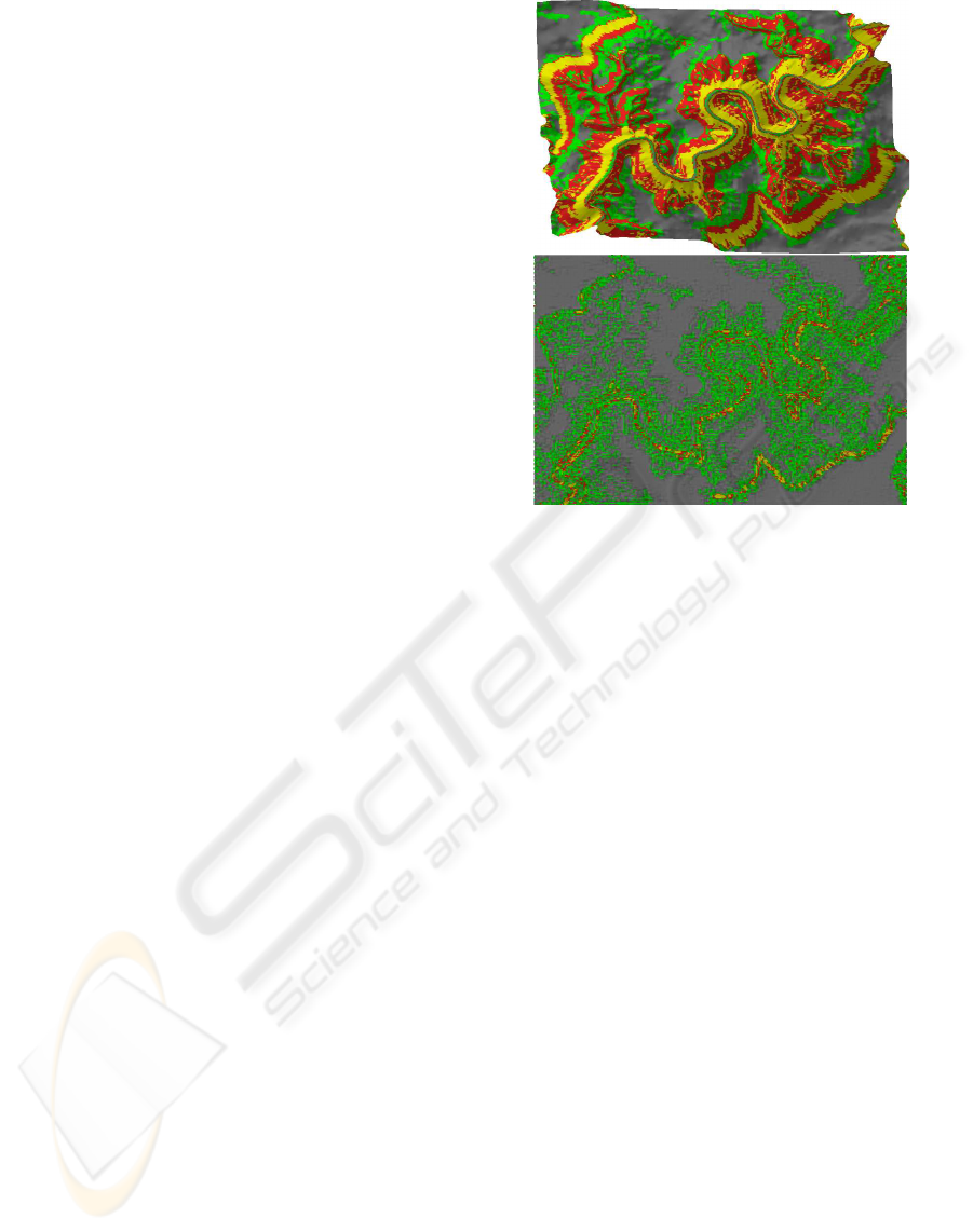
Figure 1: Top is a valley in Nevada, USA. Bottom is the

result of extracting one level of details and applying them to

a ﬂat surface. The features in the terrain clearly correspond

to features in the details. Colored by slope steepness.

Once a mapping has been speciﬁed we rearrange

the target’s row and column details into the order de-

termined by the mapping. Subdivision is used to ap-

ply the details to the rows and then the columns of

the base, doubling its resolution, producing our syn-

thesized result. This process is referred to as applying

one level of details or as performing one iteration of

subdivision.

Now consider the case where the target terrain has

a much higher resolution than the base terrain. In this

case we perform reverse subdivision to the target sev-

eral several times, until the target has approximately

the same resolution as the base. As before our next

step is to perform matching between the base and tar-

get terrains, and then subdivide the base terrain using

the last set of details extracted from the target. We

use the last set since these are the details that will de-

scribe the difference between the base’s current reso-

lution and double this resolution. We can then repeat

this matching and subdividing until we have used up

all the details in reverse order and our synthesized ter-

rain has the same resolution as the original target.

5.1 Multi-Fractals By-Example

Another way of creating terrain by-example is with

multi-fractals. This technique has drawbacks but pro-

vides another method of creating terrains by-example.

The difference between fractal terrains and multi-

fractal terrains is that the fractal scale changes over

the terrain producing terrains that are less homoge-

TERRAIN SYNTHESIS BY-EXAMPLE

125

neous. To produce multi-fractals by example we need

to capture the fractal scale from the target terrain. To

do this we must determine an estimate of the fractal

scale and use this parameter on the feature-mapped ar-

eas of the base terrain. Losasso and Hoppe (Losasso

and Hoppe, 2004) have obtained fractal scale esti-

mates for entire terrains by using the variance of

residuals. The residuals used are essentially the de-

tails resulting from linear interpolation.

In our work we estimate the fractal scale in a sim-

ilar manner. We use Miller’s Chaikin based terrain

fractals (Miller, 1986), consequently the fractal scale

becomes the variance of the displacements created by

the Chaikin details. To implement our by-example

multi-fractals we use this estimate of fractal scale over

small areas of the target and then use these to decide

the fractal scale on mapped areas of the base terrain.

With multi-fractals by-example, instead of creating

the detail quilts, we estimate residuals over the target

terrain’s selected blocks (the small area over which

the fractal scale is calculated) and store the fractal

scales to be used on the base terrain. The mapping

procedure (matching similar pieces of terrain) is still

performed, making this algorithm execute at approxi-

mately the same speed as MRA by-example.

Multi-fractals by-example have a major drawbacks

in applying small-characteristic features. To under-

stand why we must examine the generation of the

fractal displacement. For our multi-fractals we are

taking the variance of the details and using this to

scale Gaussian noise. By doing this we are discard-

ing an accurate and real distribution of details from

the target, and replacing this with a Gaussian distrib-

ution. In essence we are discarding most of the noise

we have gone to the trouble of extracting from the tar-

get. This is one of the reasons why multi-fractal by-

example results tend to resemble the target less than

MRA by-example results.

5.2 Mapping Terrain Features

The goal of this section is to ﬁnd a mapping between

similar areas and features on the target and base ter-

rains. We have made use of two existing techniques

for handling this problem. The ﬁrst is interactive, re-

lying on human interpretation to solve the matching

problem. The other technique is automatic and based

on Texture Quilting (Efros and Freeman, 2001). We

chose this technique because of its speed and quality.

5.2.1 Interactive Mapping

The simplest technique of solving the mapping prob-

lem is to leave it up to the user. We replace the guess-

ing at assorted parameters required for fractal synthe-

sis or erosion simulation with a more intuitive mech-

anism. This mechanism is having the user perceive

similar areas in the base and target terrains.

In this system the user selects a section of the target

terrain and then a section of the same size of the base

terrain. These sections may have any shape; we have

chosen to use rectangles in our system for speed of

calculation and ease of implementation. If mapped-to

areas on the base terrain already posses details we re-

place the existing details. The user can also specify

the number of levels of details to copy. The number

of levels to copy is dependent on the desired resolu-

tion but in our tests we have found that copying three

levels of detail provides good results. An example of

this process can be seen in Figures 2 and 3.

Performing the MRA is very fast (Samavati and

Bartels, 1999), allowing users to easily and quickly

see the results of their speciﬁed mapping. This inter-

active method can also be used to edit the details of

an existing terrain. By specifying a new mapping of

an area, the base terrain’s details are replaced, chang-

ing the small-scale characteristics of the selected area.

This method also easily allows more than one target

terrain to be used to reﬁne a single base terrain.

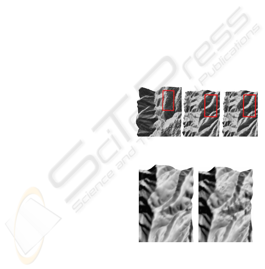
Figure 2: The interactive system copied the bumpy details

from the highlighted area of the target (left) changing a

smooth area of the base terrain (middle) into a more rough

area (right).

Figure 3: Close-up of the terrain in Figure 2, before (left)

and after (right) synthesis. The red lines have been removed

to allow examination of the borders.

5.2.2 Automatic Mapping: Terrain Quilting

In order to reduce the amount of user interaction we

have also created an automatic mapping system. This

automatic system is based on the Image Quilting al-

GRAPP 2006 - COMPUTER GRAPHICS THEORY AND APPLICATIONS

126

gorithm (Efros and Freeman, 2001) used for texture

synthesis and texture transfer.

The ﬁrst step is to break the base terrain into blocks.

We do this by dividing the base terrain into a grid

of overlapping square blocks. By choosing a smaller

block sizes, smaller features are matched and better

mappings can be produced; however, this also in-

creases the time required for the algorithm to run.

Our default setting uses blocks that are approximately

one-ﬁfteenth of the average of the base terrain’s width

and length, however, the block size is adjustable by

the user. For the best possible results the block size

should be determined by the resolution of the small-

scale characteristics the user desires to capture.

For each block in the base terrain we attempt to

ﬁnd a similar block in the target terrain. This is done

by testing the similarity of some number of randomly

selected blocks in the target. The number of candidate

blocks we test is the smaller of forty or the number of

blocks that ﬁt equally into the target. This gives a

good trade off between speed and quality, however if

poor matches occur this setting is user adjustable.

In the Image Quilting algorithm (Efros and Free-

man, 2001), the difference (or conversely the simi-

larity) between two blocks is described by the sum

of squares between the pixel brightness values. For

terrains, the values we are comparing are elevations

rather than pixel brightness so we more concerned

with features (e.g., a mountain peak in the base ter-

rain should be mapped to a mountain peak in the tar-

get terrain). Consequently, we need to examine the

shape portrayed by the block, rather than the absolute

height values of the block.

The metric we created to calculate the difference in

shape between two blocks, i from the base, and j from

the target, where we have indexed the height values in

the blocks with a single index, is:

i,j

k=1

((i

− m

) − (j

− m

))

where n is the number of height values per block, i

is the k

height value of block i, and m

is the mean

height value of block i. Unlike Image Quilting, when

calculating the difference between blocks we ignore

the blending between blocks (since we are copying

details, not pieces of terrain) so this does not con-

tribute to the difference calculation.

5.2.3 Constructing the Detail Quilts

Once we have found the best match for each base ter-

rain block, we construct a quilt of the target’s details.

This is done for both the row and the column details.

We quilt the details, rather than the actual height val-

ues, because we want a new synthesized terrain, not a

terrain that was created through mixing and matching

pieces of the target. A mix and match terrain would

suffer block blending issues and could alter large-

scale characteristics of the base terrain. Instead, the

system quilts the details so that the resulting terrain

contains merely the addition of the details from the

target. In Image Quilting a minimum error boundary

cut is used to blend overlapping areas. In our work we

use a linear blend of the details between the blocks.

We do this because details are small in respect to the

curve presented by the low-resolution data for the rea-

son described in Section 4.

6 TERRAIN RENDERING

Rendering in our system is not just a matter of sim-

ply displaying terrains. Rather it is a tool that can al-

low us to more easily evaluate, compare, and contrast

synthetic terrains. This is especially important when

presenting synthesis results in one or two images. We

use four rendering techniques that provide easier dis-

crimination between and evaluation of terrains.

Our standard rendering method uses Gouraud shad-

ing on grey colored triangles to maximize contrast and

make terrain evaluation possible when the images are

printed in black and white.

The second rendering style uses Gouraud shad-

ing but with triangles colored based on elevation.

From lowest elevation to highest triangles are colored

brown, green, red, orange, yellow, and white. This

coloring makes the terrain easier to understand, espe-

cially when the terrain is viewed from the top.

We also desired to make it easier to determine how

smooth (or rough) a terrain is. To do this we color

based on slope steepness. This is the rate of change

in elevation making it a good measure to indicate the

smoothness of a terrain (Shary et al., 2002). In our

slope steepness ﬁgures, from most steep to least steep,

the triangles are colored yellow, red, green, or grey.

We have found this gives good insight into the amount

of heterogeneity of rendered terrains and can empha-

size features such as the riverbed in Figure 1.

Our last technique uses a non-photorealistic render-

ing technique to place small ink strokes. This render-

ing technique uses silhouette stability edges with the

direction of the edge changed to point in the tangent

direction as described in Brosz’s work (Brosz, 2005).

For evaluating terrains, this rendering technique em-

phasizes the differences between rough and smooth

areas of synthesized terrains.

7 RESULTS AND DISCUSSION

There are several criteria for the success of our sys-

tem. The most important is that the synthesized ter-

rain should appear more detailed than if the base

TERRAIN SYNTHESIS BY-EXAMPLE

127

Base

First Target Second Target

First Result Second Result

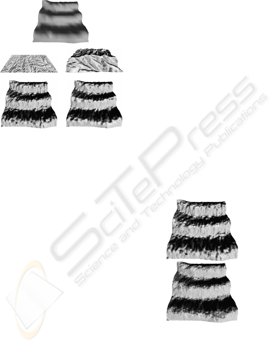
Figure 4: The ﬁrst trial. The base is a user created 20 × 20

terrain. The results are 146 × 146, produced by copying

three levels of details from their respective target terrains.

was subdivided without details. Our next expecta-

tion is that the terrain gains detail in a manner that

is more predictable and realistic than current proce-

dural methods. A related point is that we expect the

synthesized terrain to show small-scale characteristics

similar to those of the target. Another important goal

for the success of the system is in the simplicity of the

user interaction.

7.1 Providing a Control Synthesis

To compare the results of the terrain by-example sys-

tem to the results of a fractal-based synthesis, we im-

plemented fBm subdivision as described by Miller

(Miller, 1986) with Voss’ successive random addi-

tions (Peitgen and Saupe, 1988) to further reduce frac-

tal artifacts. We estimate the initial fractal scale based

on our residual calculation. H, the parameter control-

ling the change in fractal scale (Fournier et al., 1982),

is 0.85 as we found this value produces good results.

We have not considered erosion techniques due to

two problems. The ﬁrst is that they involve many pa-

rameters that must be provided. These parameters

depend on the type of terrain as well as many envi-

ronmental conditions. The other is that these erosion

simulations are likely to remove or signiﬁcantly alter

previously existing features of the base terrain that are

real features and desired in the resulting model.

7.2 Experimentation

In this subsection we present two trials using Chaikin

MRA. In the ﬁrst trial we synthesized a terrain from a

small, low resolution, hand-made terrain. The second

trial compares a real, high-resolution terrain with a

synthesized terrain that uses low resolution data from

the same area as its base terrain. In both trials we

used the default block size. Timings were performed

on an AMD 2600XP+ with 1.5GB RAM and an ATI

9800 128MB video card. The base and target terrains

used in our ﬁrst trial, as well as the terrains resulting

from our synthesis, are shown in Figure 4. The ﬁrst

target is a 30m NED from Kansas, USA, the second

is a 30m NED from Utah, USA. The base terrain’s

resolution was increased from approximately 240m

to 30m resolution. Figure 5 compares the result of

fBm fBm synthesis to a result achieved with terrain

by-example synthesis. The terrain by-example syn-

thesis in this trial took approximately 3 seconds while

the fBm synthesis required less than 1 second.

In comparing our two synthesized results, we can

see that changing the target signiﬁcantly changes the

synthesis result. The ﬁrst result has more jagged fea-

tures, similar to the jagged hills in the Kansas target

whereas the second result is smoother, more like the

Utah target. Looking at our results, especially the

sides of the hills, we can see that they have interesting

bumps added while also appearing smooth, much like

the target terrains. In contrast, the fBm result is very

rough all over. The fBm synthesis, because it changes

the height at random is uniformly noisey, whereas the

by-example results are more coherent.

Figure 5: Trial 1 comparison between by-example (top) and

fBm synthesis (bottom). Notice the homogeneous nature

fBm result when compared to the by-example result.

Our second trial uses a 30m NED of an area within

the Utah salt ﬂats as its base terrain. We chose a 10m

NED from another portion of the Utah salt ﬂats as our

target (shown in Figure 6). The base and the results

of by-example and fBm synthesis are shown in Figure

GRAPP 2006 - COMPUTER GRAPHICS THEORY AND APPLICATIONS

128

7. Figure 8 provides comparison between 10m NED

data of the same area and the two synthesized 7.5m

results. The by-example result (2794× 394), obtained

from two levels of copied details, was created in 8

seconds; the fBm result required 2.5 seconds.

In Figure 7 our synthesized terrain shows very lit-

tle introduced roughness. This is due to the smoothed

nature of the NED as well as the smooth nature of

the salt ﬂats. Close inspection reveals small irregu-

larities added to several of the mountain ridges and a

few small bumps in the ﬂat area. In the fBm terrain

we see that the introduced noise obscures some of the

streambeds in the middle of the terrain. The most no-

ticeable difference is that the fBm synthesis adds a

large number of undesirable bumps to the ﬂat area.

This trial, with the mountainous terrain at one end

and the very ﬂat terrain at the other, emphasizes the

drawback of fBm synthesis. The estimated fractal

scale is the average residual from the entire terrain,

resulting in terrain that is too rough at the ﬂat end and

too smooth at the other. Use of multi-fractals could

ﬁx this, but even then the scale is still estimated over

some area and, if that area has heterogeneous fea-

tures, the scale can again be wrong. MRA however,

is based on wavelets that are able to capture and rep-

resent these different scales effectively.

It is important to note that the ﬂats cannot be syn-

thesized in a better fashion by simply adding erosion

to the fBm synthesis. Thermal weathering erosion

(Musgrave et al., 1989) may somewhat reduce the size

of the fractal bumps, but not completely because the

bumps are small and have very little slope. Hydraulic

erosion techniques can smooth these bumps out but

are designed to, and will, introduce new rivers and

valleys, destroying the features of the base terrain.

7.3 Chaikin vs Multi-Fractals

In Section 5 we have discussed two different tech-

niques of extracting and applying details. Chaikin

MRA, is useful because it is based on third order B-

Splines that effectively capture the smooth underlying

nature of terrains. Multi-fractals by-example provide

a close link to existing procedural methods. To com-

pare these techniques we have repeated the ﬁrst trial

using multi-fractals. Figure 9 shows the results.

In Figure 9 it is clear that the multi-fractals are not

as successful in capturing the character of the target

terrain. It is not clear that the left multi-fractal re-

sult came from the ridge-ﬁlled Kansas target while

the right came from Utah target. The Chaikin MRA

results show these differences.

7.4 Texture Transfer Compared

An important topic is why current texture transfer

techniques are not suitable for synthesizing terrain. In

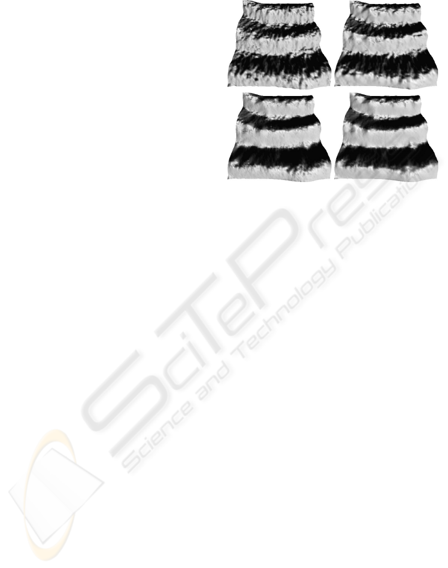
Figure 9: Repeat of Trial 1 (Figure 4) with Chaikin MRA

(top) and multi-fractals by-example (bottom). In the left

column are the results that used Kansas target, the right col-

umn presents the results of the Utah target.

some senses they are suitable. Can a target terrain be

broken into pieces and then sewn together to form a

realistic terrain or, as in Image Analogies, two differ-

ent resolutions of the target terrain could provide a

ﬁlter to increase the resolution of the base terrain?

The difference between our method and texture

transfer approaches is that we do not copy pieces of

terrain; instead we copy details. This ensures that our

result is composed mostly of the features of the base

terrain. Texture transfer rearranges pieces of the tar-

get to ﬁt the base, making these methods unsuitable

for increasing the resolution of existing terrain. By

using details, since they are such small contributions

to the result, we also avoid the blending artifacts that

appear in texture transfer methods.

To test this we compare a terrain synthesized by-

example with results of two texture transfer systems:

Image Quilting (Efros and Freeman, 2001) imple-

mented by Robert Burke (Burke, 2005) and the Image

Analogies system (Hertzmann et al., 2001). Figure 10

shows the base, target, and our synthesis.

To perform the Image Quilting texture transfer, we

convert the DEM to a height encoded image (i.e., an

image where the highest areas are white and the low-

est are black). Next, we resample the 30m base to a

10m resolution. This is akin to subdividing without

adding details, producing a smooth, high-resolution

terrain. We then apply texture transfer between the

target and the resampled base producing the result

shown in Figure 11. It is clear that directly using

the original terrain has introduced blending problems,

failing to produce a realistic terrain.

For the Image Analogies texture transfer we used

height encoded images of the 30m and 10m NED

target terrain as the learning pair. As both of these

images had to be the same size, we resampled the

TERRAIN SYNTHESIS BY-EXAMPLE

129

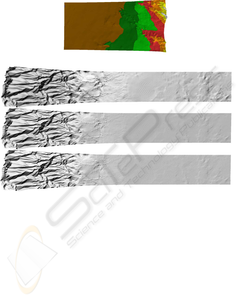
Figure 6: The target terrain used in the second trial, colored by elevation. This is a 10m NED from the Utah Salt Flats.

Figure 7: The second trial. The top image is the base terrain (30m NED data from the Utah Salt Flats), the middle is the

Chaikin, terrain by-example result, and the bottom is the result of fBm synthesis.

30m image to achieve 10m resolution. Similarly the

30m base image was also resampled. The chossen

matching method was Hertzmann et. al’s recom-

mended approximate nearest neighbor search. Figure

11 presents our best result with this system. More

results of our testing can be seen in Brosz’s work

(Brosz, 2005). The result of the Image Analogies

system does not reproduce the ﬂat area of the upper

left base terrain and generally produces terrains with

a speckled appearance. The hillsides have new ridges

and lines, giving an interesting but unwelcome ter-

raced look. It does not appear to be a bad result un-

less one considers that neither the base nor the target

has these features. Both terrains have ridges but these

ridges are mostly smooth, not noisy like synthesis re-

sult. Since neither the base nor the target terrains have

speckles, these must be artifacts created by blending

problems when placing pixels.

The results of two texture transfer systems show

that they have problems in maintaining ﬂat terrain due

to the problems of blending images (as opposed to

blending details). It is also due to the fact that they

are designed to preserve the source image (the target

terrain) rather than to keep the features of the target

image (the base terrain). The Image Analogies system

performed better than the Image Quilting system but

overall we feel it is clear that terrain by-example is

superior for synthesizing terrain.

8 CONCLUSIONS

In this work a pipeline to synthesize terrains based on

an example terrain has been presented. This system

simpliﬁes user interaction, replacing procedural and

erosion parameters with selection of a target terrain.

The resulting terrains show inﬂuence from the target

terrain and have heterogeneous features. Lastly the

synthesis is completed quickly, achieving synthesis in

seconds. The availability of high resolution terrain

GRAPP 2006 - COMPUTER GRAPHICS THEORY AND APPLICATIONS

130

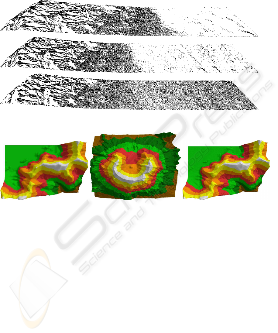
Figure 8: Non-photorealistically rendered comparison between the real, 10m resolution NED (top), our second trial’s 7.5m

by-example result (middle), and the 7.5m result of fBm synthesis (bottom). Notice the roughness of the salt ﬂat fBm result.

Figure 10: The left image is of the base terrain (30m NED of Harmony Flats, Washtingon, USA), the middle is the target

(10m NED of Mount St. Helens, Washington, USA) and the bottom is the by-example synthesis result.

data for use as targets makes this system possible.

In examining our criteria for success, we can see

that our synthesised terrains are more detailed than

the base terrain. Moreover, the terrains gain details

that seem realistic. This is shown in all the trials,

but particularly in Trial 2 where the by-example re-

sult maintained the ﬂatness of the salt ﬂats. The in-

teractive system copies details from the target to the

base in a predictable manner. The automatic sys-

tem also results in terrains that show characteristics of

the target terrain (Figure 4). The by-example results

appear similar to even if they do not exactly match

the real, high resolution data of the same area. Our

system simpliﬁes user interaction, producing user-

speciﬁed terrain without input of a plethora of para-

meters. By-example synthesis can create completely

synthetic terrains as well as add levels of detail to ex-

isting terrain.

Multi-resolution analysis provides an efﬁcient and

effective method for capturing and copying the char-

acter of a terrain. Multi-fractals present another

method of extracting details from the target terrain,

however this technique is unable to capture a target’s

character as well as Chaikin MRA.

Both the interactive and the automatic methods

provide good starting points for feature matching in

this pipeline. The techniques work well for most ter-

rains, however, both methods have drawbacks. The

interactive method requires more input from the user.

For large terrains this could become time consuming

and tedious. However, this system offers the potential

for editing of existing details in terrains that proves an

interesting and potentially useful feature.

The automatic feature mapping system has several

limitations. Our random block matching technique,

adapted from Image Quilting, is not ideal because

it does not guarantee that the best matching block

in the target terrain is found. An exhaustive search

or variation of simulated annealing could ensure bet-

ter matching. From our examination of the matches

made by our system it seems that the current system

works well without modiﬁcation. Other techniques

for comparing shapes could increase the effectiveness

or speed of automatic matching.

TERRAIN SYNTHESIS BY-EXAMPLE

131

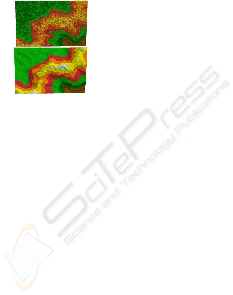
Figure 11: Top is the result of the Image Quilting algorithm

using settings of 3 iterations, initial block size of 16, 17%

overlap, and 50 candidates. Bottom is a result of the Image

Analogies algorithm using steered ﬁlters and the default set-

tings. Both are rendered with elevation coloring.

There is also the issue of how the block size should

be chosen. Small block sizes can achieve more ac-

curate matches, but when the block size is too small,

neighboring information is lost, causing bad matches.

The values we have used produce qualitatively good

results, however, a more quantitative examination

would be useful. Adding a contribution from the

neighboring area to the error metric might also alle-

viate the small block problem.

8.1 Future Work

Introducing a painting interface to specify speciﬁc

mappings could increase the functionality of the by-

example system. This could be similar to the paint

by numbers used with Image Analogies (Hertzmann

et al., 2001). This could make it easier for users to

indicate mappings and to specify different target ter-

rains. E.g., half a base terrain could be painted yel-

low, with yellow mapped to a desert target, and the

rest could be mapped to a mountainous target.

There exist methods (Pumar, 1996), (Brivio and

Marini, 1996) that use estimates of fractal dimension

(opposed to our estimate of fractal scale) to increase

the resolution of terrains. It is possible that these al-

ternative estimates may improve the quality of the ter-

rain synthesized with multi-fractals by-example. It is

our intuition however, that the poor performance of

multi-fractals is more greatly due to the randomness

of displacements as opposed to the size of those dis-

placements. Consequently, we are not optimistic of

improving the multi-fractal by-example technique.

Triangulated Irregular Networks (TINs) abandon

the regular grid format of DEMs, reducing the number

of data points necessary to represent terrains. TINs

are able to better represent sharp features, such as

ridges, by aligning triangle edges with feature edges

(DEM’s edges seldom coincide with features). A

more sophisticated shape analysis technique in con-

junction with the details extracted with progressive

meshes (Hoppe, 1996), arbitrary topology MRA, or

another multi-resolution technique could create a TIN

by-example system.

REFERENCES

Benes, B. and Forsbach, R. (2001). Layered data repre-

sentation for visual simulation of terrain erosion. In

Proceedings of SCCG ’01, pages 80–86.

Brivio, P. A. and Marini, D. (1996). A fractal method for

digital elevation model construction and its applica-

tion to a mountain region. Computer Graphics Forum,

12(5):297–309.

Brosz, J. (2005). Terrain modeling by example. Master’s

thesis, University of Calgary, Department of Com-

puter Science.

Bryce (2005). Bryce 5.0 User Manual. Daz Software. http://

bryce.daz3d.com/Bryce5

Manual DAZ.pdf.

Burke, R. (2005). Image quilting, texture transfer, and wang

tiling implementation. http://www.heroicsalmonleap.

net/mle/wang/.

Chiang, M., Huang, J., Tai, W., Liu, C., and Chang, C.

(2005). Terrain synthesis: An interactive approach.

In International Workshop on Advanced Image Tech.

Ebert, D. S., editor (1994). Texturing and Modeling: A Pro-

cedural Approach. AP Professional.

Efros, A. A. and Freeman, W. T. (2001). Image quilting

for texture synthesis and transfer. In Proceedings of

SIGGRAPH ’01, pages 341–346.

Fournier, A., Fussell, D., and Carpenter, L. (1982). Com-

puter rendering of stochastic models. Commun. ACM,

25(6):371–384.

Garland, M. and Heckbert, P. S. (1997). Surface simpliﬁ-

cation using quadric error metrics. In Proceedings of

SIGGRAPH ’97, pages 209–216.

Hertzmann, A., Jacobs, C. E., Oliver, N., Curless, B., and

Salesin, D. H. (2001). Image analogies. In Proceed-

ings of SIGGRAPH ’01, pages 327–340.

Hoppe, H. (1996). Progressive meshes. In Proceedings of

SIGGRAPH ’96, pages 99–108.

Kelley, A., Malin, M., and Nielson, G. (1988). Terrain sim-

ulation using a model of stream erosion. In Proceed-

ings of SIGGRAPH ’88, pages 263–268.

Lewis, J. P. (1987). Generalized stochastic subdivision.

ACM Transactions on Graphics, 6(3):167–190.

Losasso, F. and Hoppe, H. (2004). Geometry clipmaps: ter-

rain rendering using nested regular grids. ACM Trans-

actions on Graphics, 23:769–776.

GRAPP 2006 - COMPUTER GRAPHICS THEORY AND APPLICATIONS

132

McLusky, J. (2005). Terrain dialog description. http://www.

planetside.co.uk/terragen/guide/dlg

terrain.html.

Miller, G. S. P. (1986). The deﬁnition and rendering of ter-

rain maps. In Proceedings of SIGGRAPH ’86, pages

39–48.

Musgrave, F., Kolb, C., and Mace, R. (1989). The synthesis

and rendering of eroded fractal terrains. In Proceed-

ings of SIGGRAPH ’89, pages 41–50.

Nagashima, K. (1997). Computer generation of eroded val-

ley and mountain terrain. The Visual Computer, pages

456–464.

Peitgen, H.-O. and Saupe, D., editors (1988). The Science

of Fractal Images. Springer-Verlag.

Pumar, M. A. (1996). Zooming of terrain imagery using

fractal-based interpolation. Computers and Graphics,

20(1):171–176.

Roettger, S. and Frick, I. (2002). The terrain rendering

pipeline. In Proc. of East-West Vision ’02, pages 195–

199.

Samavati, F. F. and Bartels, R. H. (1999). Multiresolution

curve and surface representation by reversing subdivi-

sion rules. Computer Graphics Forum, 18(2):97–120.

Samavati, F. F. and Bartels, R. H. (2004). Local bspline

wavelets. In Proceedings of the International Work-

shop on Biometric Technologies 2004.

Schroeder, W. J., Zarge, J. A., and Lorensen, W. E. (1992).

Decimation of triangle meshes. In Proceedings of

SIGGRAPH ’92, pages 65–70.

Shary, P. A., Sharaya, L. S., and Mitusov, A. V. (2002). Fun-

damental quantitative methods of land surface analy-

sis. Geoderma, 107(1-2):1–32.

Simoncelli, E. P., Freeman, W. T., Adelson, E. H., and

Heeger, D. J. (1992). Shiftable multi-scale transforms.

IEEE Trans. on Informations Theory, 38(2):587–607.

U.S.G.S. (2005). Seamless data distribution system.

http://seamless.usgs.gov.

TERRAIN SYNTHESIS BY-EXAMPLE

133