
RELIABLE COMPUTATION OF ROOTS TO RENDER REAL
POLYNOMIALS IN COMPLEX SPACE
∗
J.F. Sanjuan-Estrada, L.G. Casado and I. Garc
´
ıa
Departament of Computer Archictecture and Electronic
University of Almeria
Ctra Sacramento s/n, 04120, Almeria (Spain)
Keywords:
Computational geometry, Complex roots of real polynomials, Video sequences in complex space.
Abstract:
Many geometric applications involve computation and manipulation of non-linear algebraic primitives. These
basic primitives like points, curves and surfaces are represented using real numbers and polynomial equations.
For example, ray tracing technique rendering three-dimensional realistic images, where each pixel need to
find the minimum positive root of intersection point when a lineal ray hit a surface. However, the intersection
between a ray and a polynomial equation has differents roots, where each root can be a real number (without
imaginary part) or a complex number (with real and imaginary part), so that, the number of roots is equal to
degree of polynomial.
In this paper, we extend the traditional ray tracing technique to show roots in the complex space. We use an
algorithm that analyse all verified roots of intersection point using interval arithmetic. This algorithm computes
verified enclosures of the roots of a polynomial by enclosing the zeros in narrow bounds. The reliability of the
algorithm depends on the accurate evaluation of these complex roots. Finally, we propose differents solutions
to render a image in the complex space, where the arguments of complex roots are used to choose the roots
of intersection point in complex space, while the color of each pixel is computed by minimum modulus of
complex roots chosen.
1 INTRODUCTION
Nowadays, there are several methods in computer
graphic which allow to design realistic images. These
images are composed of many different primitives,
where it is very typical the use of polynomial forms.
Usually these algorithms need to find real roots of
polynomials. For example, ray tracing techniques
need to find the minimum positive real root where a
lineal ray hits a surface.
Nevertheless, many mathematician and physician
work in the complex space, they usually plot the roots
in the two-dimensional complex plane, like Nyquist
diagram. The plane of complex number uses the x-
axis as the real axis and y-axis as the imaginary axis.
Every complex number is represented by an unique
point in the complex plane. Historically, the geomet-
ric representation of a complex number as a point in
the plane was important because it made the whole
∗
This work has been partially supported by the Ministry
of Education and Science of Spain through grants TIC2002-
00228 and TIN2005-00447
idea of a complex number more acceptable. In partic-
ular, this visualization helped ”imaginary” and ”com-
plex” numbers become accepted in mainstream math-
ematics as a natural extension to negative numbers
along the real line.
In this paper, we propose to extend the ray tracing
technique from the real space to the complex space.
This procedure leads to produce three-dimensional
images where each pixel has information about com-
plex roots of intersection point. We need reliable
algorithms that work with complex numbers to find
every roots (Georg, 1990; Gruner, 1987). After com-
puting a first approximation of each root, its error is
enclosed using interval arithmetic. If the diameter of
the error interval is less than a desired accuracy, then
a verified enclosure of the solution is given by the ap-
proximation of root and the enclosure of its error.
The rest of the paper is organized in the following
manner. An overview of a root finder algorithm that
can compute all the roots of a univariate polynomial
with the desired accuracy is given in Section 2. This
algorithm uses an iterative scheme that starts with an
initial approximation of all the roots, refines them and
305
F. Sanjuan-Estrada J., G. Casado L. and García I. (2006).
RELIABLE COMPUTATION OF ROOTS TO RENDER REAL POLYNOMIALS IN COMPLEX SPACE.
In Proceedings of the First International Conference on Computer Graphics Theory and Applications, pages 305-312
DOI: 10.5220/0001355603050312
Copyright
c
SciTePress

updates the error bound. The procedure to extend the
original ray tracing technique to the complex space is
described in Section 3. This new technique allows us
to build a three-dimensional animation of the evolu-
tion of the complex roots. In Section 4, several exam-
ples of the distribution of complex roots of polynomi-
als are shown. We conclude in Section 5.
2 ALGORITHM TO FIND
COMPLEX ROOTS OF
POLYNOMIAL
A polynomial of degree n has n different zeros. These
zeros can be real and/or imaginary roots. Finding
these roots is a non trivial problem in numerical math-
ematics. Most algorithms only deliver approxima-
tions of the exact zeros without any or with only weak
statements concerning the accuracy.
p(z) =
n
X
i=0
p
i
· z
i
, p
i
∈ R (1)
In this paper, we use an algorithm, proposed by
Hammer et al. in (Hammer et al., 1995), that com-
putes verified enclosures of the roots of a polynomial
by enclosing the zeros in narrow bounds. This algo-
rithm is based on the fact that the roots of the poly-
nomial of degree n match the eigenvalues of the com-
panion matrix A since
p(z) = (−1)
n
· p
n
· |A − z · I| (2)
where I is the identity matrix of dimension n and
A =
0 · · · 0
−p
0
p
n
1
−p
1
p
n
.
.
.
.
.
.
1
−p
n−1
p
n
(3)
2.1 Eigenvalue Problem
Hence, the problem of finding a zero of the polyno-
mial p is equivalent to find an eigenvalue z
∗
of the
matrix A. We solve the eigenvalue problem A · q
∗
=
z
∗
· q
∗
, that is f(x) = (A − z
∗
I) · q
∗
= 0, where
q
∗
is an eigenvector corresponding to the eigenvalue
z
∗
consisting of the coefficients q
∗
0
, q
∗
1
, . . . q
∗
n−1
of de-
flated polynomial:
q
∗
(z) =
n−1
X
i=0
q
∗
i
· z
i
=
p(z)
z − z
∗
(4)
Additionally, the coefficients of the deflated poly-
nomial can be determined recursively by Horner’s
evaluation of the polynomial p at the point z
∗
(C. Sid-
ney Burrus and S.Treitel., 2003):
q
∗
n−1
= p
n
q
∗
i−1
= q
∗
i
· z
∗
+ p
i
, i = n − 1, · · · , 1.
(5)
We have a system of nonlinear equations in the n
unkowns q
∗
0
, q
∗
1
, · · · , q
∗
n−2
and z
∗
. Let the vector q be
the first n − 1 components of the desired eigenvector
q = (q
∗
0
, q
∗
1
, · · · , q
∗
n−2
)
T
. The eigenvalue z
∗
often is
stored as the n
th
component of a vector (q, z)
T
.
2.2 Iterative Approach
Let f be a nonlinear and differentiable function.
A well known strategy to solve a nonlinear system
f(x) = 0 is the simplified Newton iteration using the
fixed-point form of the problem. Let a starting ap-
proximation x
(0)
be given, let R = f
0
x
(0)
−1
, and
iterate according to:
g(x
(k)
) = x
(k+1)
= x
(k)
−R·f(x
(k)
), k = 0, 1, · · ·
(6)
If x
(0)
is close to the fixed-point x
∗
, the sequence
of x
(k)
for k → ∞ approaches the fixed-point x
∗
=
g(x
∗
) with f(x
∗
) = 0.
For numerical stability reasons, it is better to per-
form a residual correction (∆), so then x = ˜x + ∆
x
.
This means that the Newton iteration has the form
x
(k+1)
− ˜x = x
(k)
− ˜x − R · f(x
(k)
), that is:
∆
(k+1)
x
= ∆
(k)
x
− R · f(˜x + ∆
(k)
x
) (7)
Hammer et al. applied the simplified Newton itera-
tion to the eigenvalue problem, where x = (q, z)
T
,
and solved the eigenvalue problem for the interval
version of Newton’s iteration algorithm in (Hammer
et al., 1995):
g
[]
([∆
x
]) = −[R] · [d] + [R] · [∆
z
] ·
[∆
q
]
0
(8)
where [R] = f
0
[x
(0)
]
−1
= [J]
−1
f
is the inverse of
the interval Jacobian matrix, and [d] = ([A] − [˜z] ·
[I]) · [q]
∗
.
2.3 The Approximate Iteration
We must determine good approximations of the ex-
act eigenvector q
∗
and eigenvalue z
∗
to avoid infla-
tion effects using the interval version of the Newton
iteration. For this purpose, we first use a non-interval
residual iteration algorithm starting with an arbitrary
starting approximation ˜z for a root of p(z). The ini-
tial eigenvector ˜q corresponding to that eigenvalue ˜z
GRAPP 2006 - COMPUTER GRAPHICS THEORY AND APPLICATIONS
306

is computed recursively by Horner’s evaluation of the
polynomial p at the point ˜z, until the corresponding
residual vector (∆
q
, ∆
z
)
T
achieves sufficient accu-
racy (C. Sidney Burrus and S.Treitel., 2003).
One of the critical steps for this iteration scheme to
work is the choice of the initial approximations to the
roots of the original polynomial.
2.4 Verification
This algorithm begins with an initial approximation ˜z
of a root of the polynomial p(z) and ˜q of the coef-
ficients of the deflacted polynomial. It improves the
approximation of a root and the coefficients of the cor-
responding deflacted polynomial to avoid overestima-
tion during the floating-point interval calculations.
The Schauder’s fixed-point theorem, which is a
generalization of Brouwer’s fixed-point theorem, is
used to get a verified enclosure of an eigenvalue of
the companion matrix A and therefore of a zero of
the polynomial (Jimenez-Melado and Morales., 2005;
Granas and Dugundji, 2004).
Schauder’s fixed-point theorem: If we have the en-
closure
[∆
x
]
(k+1)
= g
[]
([∆
x
]
(k)
) ∈ [∆
x
]
(k)
(9)
where g
[]
([∆
x
]
(k)
) is contained in the interior of
[∆
x
]
(k)
, then there exists a (not necessarily unique)
fixed-point of g
[]
and a solution x
∗
∈ ˜x + [∆
x
]
(k+1)
of the eigenvalue problem.
Subsequently, we start a new iteration step by eval-
uating the function g
[]
for a complex interval vector
argument until we achieve an enclosure (9). For com-
putational reasons, we start with a slightly inflated
approximation. The Schauder fixed-point theorem
guarantees that there exists a solution of the fixed-
point problem (9) in ([∆
q
]
(k+1)
, [∆
z
]
(k+1)
)
T
. That
is, (˜z + [∆
z
]) is a verified enclosure of an eigenvalue
z
∗
, which is a root of the complex polynomial p, and
(˜q + [∆
q
]) is a verified enclosure of a corresponding
eigenvector q
∗
, the components of which are the co-
efficients of the deflated polynomial.
2.5 Finding All Complex Roots
This algorithm proposed by Hammer et al. only find
a root in the complex space. We have extended this
algorithm, called AllCPolyZero, to find all complex
roots of the intersection point. By repeating the defla-
tion of a verified zero from the reduced polynomial,
the approximation of a new zero in the reduced poly-
nomial and the verification of the new zero in the orig-
inal polynomial, we get all complex zeros of the poly-
nomial. This extended algorithm to find all roots has
the following scheme:
AllCPolyZero
1. pdef l ated = original polynomial;
2. z = arbitrary starting for a root
3. Repeat
(a) Approximate to z a new zero of pdeflated
(b) Verify the new zero for original polynomial
(c) Deflate verified zero from pdeflated
4. Until n = degree of polynomial
2.6 Multiprecision Arithmetic
When this algorithm renders a surface, the intersec-
tion between a ray and surface can have two zeros
so close together. This happened firstly near edge
of surface. In this case, the original algorithm finds
two zeros extremely close together how a single zero.
Because, if two or more zeros of the polynomial are
so close together that they are identical in their num-
ber representation up to the mantissa length and differ
only in digits beyond the mantissa, they are called ”a
numerical multiple zero”. Such zeros cannot be ver-
ified with the program above described because they
cannot be separated by the given number representa-
tion. The program handles them just like a zero and
terminates.
If two o more zeros are extremely close together,
i.e. they form a cluster, it is not possible to verify
a zero of this cluster with the implementation given
by Hammer, because the derivative (p
0
) of the poly-
nomial p is zero. Thus, the matrix J is singular and
the inverse R cannot be enclosed because it does not
exist. We may overcome this limit of the implemen-
tation by computing the inverse of the Jacobian ma-
trix with higher accuracy. Finally, we have imple-
mented the algorithm using a multiprecision floating-
point and floating-point interval arithmetic with dou-
ble mantissa length to find close zeros and clusters of
zeros.
Once all the initial approximations are found, we
are ready to perform each step of the iteration. As
consecutive iterates are found, we need to compute
the absolute error of each approximation. For this, we
make use of a result from Smith (Smith, 1970) which
is defined by the following theorem:
THEOREM 5. Let x
(k)
1
, x
(k)
2
, · · · , x
(k)
n
be dis-
tinct and let σ
j
= f(x
(k)
j
/g
0
(x
(k)
j
) for j = 1, · · · ,
n [g(x) = Π
n
i=1
(x − x
(k)
i
)]. Define
Γ
i
: |x − x
(k)
i
| ≤ n|σ
i
|, i = 1, · · · , n (10)
Then the union of the circles Γ
i
contains all the roots
of f(x). Any connected component of this consisting
of m circles contains exactly m roots of f(x).
RELIABLE COMPUTATION OF ROOTS TO RENDER REAL POLYNOMIALS IN COMPLEX SPACE
307
We use the above results to compute the absolute
error in each iterate. The root finder algorithm pro-
ceeds as the following steps:
1. If all the circles Γ
i
are isolated, we have achieved
root isolation and if the radius of these circles is
smaller than the precision limit, we are done.
2. However, if there are clustered roots, it is possible
that some of the circles are connected. In this case
we compute the worst case error
i
= max(|x
(k)
i
−
x
(k)
j
| + n · |σ
j
|), where j ranges over the set of
indices for which x
(k)
j
is part of the same connected
component as x
(k)
i
(a) If
i
is smaller than the desired precision, we re-
port a multiple root.
(b) Otherwise, we redistribute these approximations
on a single circle with center at the centroid of
the iterates and radius equal to max
i
(
i
+ n ·
|σ
j
|), where i belongs to the iterate indices of
the same connected component of the circles.
Since all the results of our computations have guar-
anteed error bounds, we can assure the root separation
if the circles determined by the error bounds are not
connected.
3 RENDERING COMPLEX SPACE
The previous section has described our general algo-
rithm for computing every roots of a polynomial and
all the arithmetic is done in the complex space. In
this section, we will briefly describe the technique we
use to compute the color of each pixel of an rendered
image using a ray tracing technique. The traditional
ray tracing uses the minimum positive root to assign
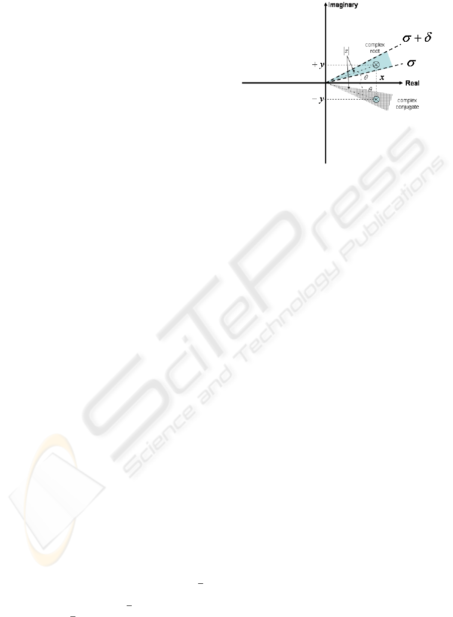
the color of a pixel in real space. A complex number
z = x + i · y can be represented in complex space,
like ρ · e
i·θ
, the magnitude represents its modulus ρ
and the angle θ its complex argument (see Figure 1).
In our algorithm the selected root is that with the
minimum magnitude and with its complex argument
θ in a selected range given by σ ≤ θ ≤ σ + δ. The
selected root will determine the final colour of a pixel.
This means that the rendering process is guided not
only by the magnitude of the roots but also it can play
with their complex arguments. This algorithm will
allow to sample the complex space, so that different
images can be obtained by choosing the interval angle
[σ, σ + δ] (see Figure 1). For example, for rendering
a scene in the real space, σ = 0 and δ = 10
−10
are
appropriate values. However, for σ = 0.1 and δ =
π
4
,
the selected roots belong to the complex space with
angles between 0.1 ≤ θ ≤ 0.1 +
π
4
and their complex
conjugate −0.1 −
π
4
≤ θ ≤ −0.1. In this case, the
real roots are not included in the search space.
Figure 1: Sampling complex space.
This procedure allows us to render three-
dimensional complex algebraic surfaces in the
complex space with an angle bounded. For rendering
all complex space using ray tracing, we can sample
all space with different values of δ and σ. Due to the
symmetry of the conjugate complex roots, it is only
necessary to sample the complex space determined
by σ ≥ 0 and σ + δ ≤ π .
When we render a scene defined by complex alge-
braic surfaces, we can use a maximum δ value equal
to π (and σ = 0). The result is that we obtain a large
amount of roots associated to the same pixel because
we are dealing with the full complex space. Our pro-
posal consists of sampling the complex space with a
narrow aperture angle; i.e. small values of δ. This
method allows us to generate an animated sequence
of images, each corresponding to a different value of
δ. The animated sequence of images gives an interest-
ing information about the distribution of roots in the
complex space.
4 EXPERIMENTATION
We use the C-XSC library, a C++ class library for
eXtended Scientific Computing, to implement the al-
gorithm proposed. Its wide range of numerical data
types, operators and functions for scientific computa-
tion makes C-XSC especially well suited as a specifi-
cation language for programming with automatic re-
sult verification.
The automatic verification of numerical results is
based on interval arithmetic. The easiest technique for
computing verified numerical results is to replace any
real or complex operation by its interval equivalent
and then to perform the computations using interval
arithmetic. This procedure leads to reliable and ver-
GRAPP 2006 - COMPUTER GRAPHICS THEORY AND APPLICATIONS
308

ified results. However, the diameter or the computed
enclosures may be so wide as to be practically use-
less. We have applied to our algorithm the principle
of iterative refinement. After computing a diameter
of the error interval is less than a desired accuracy,
then a verified enclosure of the solution is given by
the approximation and the enclosure of its error.
In order to observe the performance of our algo-
rithm, we used a set of polynomials with more than
twenty different polynomials. However, we show
only five interesting polynomials in this paper due to
space limitations (see Table 1).
Table 1: Polinomial surfaces.
Surface Coefficients of polynomial
Whitney x
2
· z + y
2
Plucker x
2
· z − x · y + y
2
· z
Bicube x
4
+ y
4
+ z
4
− 1000
Mitchell 4 · (x
4
+ (y
2
+ z
2
)
2
) + 17 · x
2
· (y
2
+ z
2
)−
20 · (x
2
+ y
2
+ z
2
) + 17
Steiner x
2
· y
2
+ x
2
· z
2
+ x · y · z + y
2
· z
2
Figure 2 shows an evolution of rendered Bicube
surface in complex space for σ = 0 in every images
and δ values from 0 (real surface in real space) to
π
9
.
This sequence of images shows how complex roots
cover the real object like packing paper. However,
if the object is a Mitchell surface, we can see that
complex roots begin covering over object. Although,
the number of complex roots around horizontal-axis
increase quicker than those around vertical-axis (see
Figure 3).
The three following sequences of images for
Steiner, Whitney and Plucker surfaces are very inter-
esting. The complex roots of these surfaces not cover
over object, but they are around imaginary axes of
surfaces. For example, the Steiner surface shows the
three axes which appear in complex space (see Fig-
ure 4) and Whitney surface has complex roots only
around one imaginary axis (see Figure 5), like Plucker
surface (see Figure 6). It is important to show that the
number of complex root increase quicker for Steiner
surface than Whitney surface.
Finally, we show a scene with a Whitney surface in-
side a translucent sphere (see Figure 7). In this case,
we have chosen to render Whitney surface like a com-
plex object and sphere like a real object. This let us
see the evolution of complex object inside a real ob-
ject for several δ values, with refraction and reflection
effects.
5 CONCLUSIONS
We have designed and implemented a complex root
finder algorithm to render polynomial surfaces in
complex space. For this problem, it is not possi-
ble to use the Sturm sequences of a polynomial as a
root finder algorithm, because we try to find complex
roots. So we solve this problem as a eigenvalue prob-
lem, where we have used the polynomial root find-
ing algorithm proposed by Hammer with some addi-
tional extras. On the one hand, we have solved how to
find close zeros of zeros with higher accuracy. On the
other hand, we have extended this algorithm to find
all complex roots in intersection point.
This algorithm also allow us to render algebraic
surfaces defined as complex polynomial, where some
of coefficients of polynomial are complex numbers.
An additional possibility it is to redefine every rays
with complex origin points and complex direction
vectors.
Finally, we propose a new procedure to render im-
age with traditional ray tracing technique in complex
space. This technique allows to build a sequences of
images where we can analyse the evolution of com-
plex root of several polynomial surfaces in a three-
dimensional space. These images can use reflection,
refraction and translucent effects like a realistic im-
age.
REFERENCES
C. Sidney Burrus, J.W. Fox, G. S. and S.Treitel. (2003).
Horner’s method for evaluating and delating polyno-
mials. Rick University.
Georg, S. (1990). Two methods for the verified inclu-
sion of zeros of complex polynomials. In Ullrich,
C., editor, Contributions to computer arithmetic and
sefl-validating numerical methods, pages 229–244.
IMACS, Scientific Publishing Co.
Granas, A. and Dugundji, J. (2004). Fixed point the-
ory. Bulletin of the American Mathematical Society,
41(2):267–271.
Gruner, K. (1987). Solving complex problems for polyno-
mials and linear systems with verified high accuracy.
In Kaucher, E., K. U. and Ullrich, C., editors, Com-
puter arithmetic, scientific computation and program-
ming languages, pages 199–220.
Hammer, R., Hocks, M., Kulisch, U., and Ratz, D. (1995).
C++ Toolbox for Verified Computing I: Basic Numer-
ical Problems: Theory, Algorithms, and Programs.
Springer-Verlag, Berlin.
Jimenez-Melado, A. and Morales., C. (2005). Fixed point
theorems under the interior condition. Procceding of
the American Mathematical Society, 134(2):501–507.
Smith, B. T. (1970). Error bounds for zeros of a polynomial
based upon Gerschgorin’s theorems. Journal of the
ACM, 17(4):661–674.
RELIABLE COMPUTATION OF ROOTS TO RENDER REAL POLYNOMIALS IN COMPLEX SPACE
309
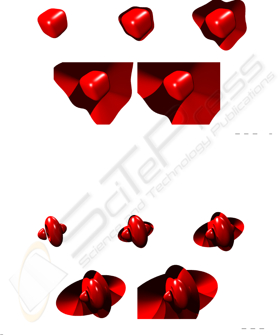
Figure 2: From up-left to down-right, Bicube surface are shown, obtained using the following δ values: 0,
π
36
,
π
18
,
π
12
and
π
9
.
All Bicube surfaces are rendering for σ = 0.
Figure 3: From up-left to down-right, Mitchell surface are shown, obtained using the following δ values: 0,
π
36
,
π
18
,
π
12
and
π
9
. All Mitchell surfaces are rendering for σ = 0.
GRAPP 2006 - COMPUTER GRAPHICS THEORY AND APPLICATIONS
310
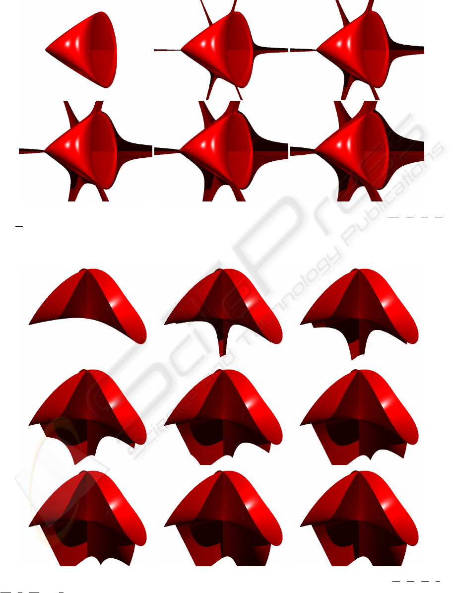
Figure 4: From up-left to down-right, Steiner surface are shown, obtained using the following δ values: 0,
π
180
,
π
90
,
π
60
,
π
45
and
π
36
. All Steiner surfaces are rendering for σ = 0.
Figure 5: From up-left to down-right, Whitney surface are shown, obtained using the following δ values: 0,
π
36
,
π
18
,
π
12
,
π
9
,
5·π
36
,
π
6
,
7·π
36
and
π
4
. All Whitney surfaces are rendering for σ = 0.
RELIABLE COMPUTATION OF ROOTS TO RENDER REAL POLYNOMIALS IN COMPLEX SPACE
311
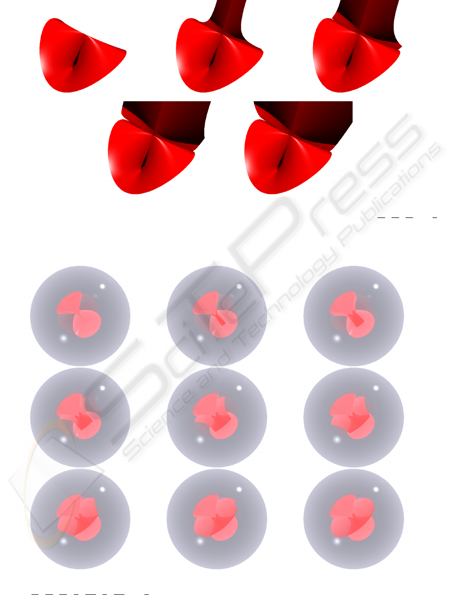
Figure 6: From up-left to down-right, Plucker surface are shown, obtained using the following δ values: 0,
π
36
,
π
18
,
π
12
and
π
9
.
All Plucker surfaces are rendering for σ = 0.
Figure 7: From u p-left to down-right, Whitney surface inside a translucent sphere are shown, obtained using the following δ
values: 0,
π
36
,
π
18
,
π
12
,
π
9
,
5·π
36
,
π
6
,
7·π
36
and
π
4
. All images are rendering for σ = 0.
GRAPP 2006 - COMPUTER GRAPHICS THEORY AND APPLICATIONS
312
