TOWARDS VISUAL-BANDWIDTH:

GETTING CLOSE TO ONE’S EXPERIMENT DATA

Mark R. Titchener

The University of Auckland

Division of Science and Technology, Tamaki Campus, Morrin Road, Private Bag, Auckland

Keywords:

information visualisation, graphical data interface, data animation.

Abstract:

This paper presents a novel general purpose visualisation environment S

(Space Odyssey), that has

evolved in relation to our research needs involving analysis and measurement of chaos and complexity in

time-series data. More speciﬁcally our attention has turned to deriving sleep state information from EEG/EOG.

operates largely as an interpreter of formated data ﬁles, to display surfaces, static and/or animated line

and point graphs, individually or simultaneously in a virtual 3-D viewing space. It comfortably handles sur-

faces of more than 100,000 vertexes, and combinations of more than 15,000 static and/or animated graphs.

User controls allow dynamic changes to viewing angle, lighting and display parameters. S

is ideally

suited to ‘scoping’ experiment data and results, for visually debugging complex processing algorithms, or

simply providing visual insight into complex data sets.

1 INTRODUCTION

This paper brieﬂy introduces S

(2005: Space

Odyssey), an interactive graphical display tool offer-

ing a combination of features tailored for scoping ex-

periment data. The name is taken from the Kubrick

ﬁlm (Clarke and Kubrick, 1968), in which animated

graphics featured with appealing simplicity as a back-

drop to many of the scenes.

A plethora of graphics oriented applications al-

ready exist! Why another? Many applications, like

Matlab (Moler, 1980), Mathematica, Maple (Char

et al., 1983), S (Becker and Chambers, 1981), and

more recently R (Ihaka and Gentleman, 1996), com-

bine numerical and programming options with a

broad range of graphical support features. Not all

research projects sit comfortably within these self-

contained computationally oriented environments.

Our own research in sleep related studies has

evolved largely within the context of UNIX. The shell

environment (Kochan and Wood, 1990), with its no-

tion of standard I/O, ﬁlters, pipes, and redirection, en-

courages a distinctive mode of work, one that places

a reliance on tools, rather than on applications. An

established range of highly optimised tools are stan-

dardly distributed with UNIX operating systems, and

may be combined within single line instructions to

achieve efﬁcient ‘one-off’ processing operations, or

saved as executable shell script ﬁles for later use.

Within this setting, we have developed and reﬁned

C-coded tools for computing complexity and entropy

from symbolic encodings of real-valued time series.

The underlying string parsing operations embody ty-

pographical rather than numerical processing not eas-

ily handled within a mathematically oriented environ-

ment. Combining these with other standard UNIX

tools enables us to compute the bulk of our results.

Our use initial of Matlab was thus limited to periph-

eral computations and graphical display of the re-

sults. With time, this mode of working presented us

with a bottleneck thus motivating the development of

is built around the OpenGL and GLUT li-

braries and operates as a stand alone tool, comple-

menting our existing computational capabilities. It

operates as an interpreter, translating static graphical

prescriptions into 3D visualisation experiences. Its

ability to accept large numbers of simple graphical

objects gives access to visual effects that are geared

to data ’scoping’. Interactive features, enable ﬂexible

animation and manipulation of the objects.

Our early focus was on improving visual-

bandwidth over a narrow range of graphical functions.

However, its capabilities have expanded considerably

378

R. Titchener M. (2006).

TOWARDS VISUAL-BANDWIDTH: GETTING CLOSE TO ONE’S EXPERIMENT DATA.

In Proceedings of the First International Conference on Computer Graphics Theory and Applications, pages 378-383

DOI: 10.5220/0001354003780383

 SciTePress

beyond the initial requirements and is broadly useful

in experimental research settings.

Separation of visualisation issues from the compu-

tational, created initially unforeseen opportunities at

the data interface and invites creative use of the data

structures both for visualisation as well as the subse-

quent data processing steps. Thus S

has con-

siderably changed the way we now undertake our re-

search.

2 SLEEP-STATE RESEARCH

Determining patient sleep-state from recorded poly-

graph time-series data, usually requires a skilled pro-

fessional, trained to recognise the salient features in-

dicative of brain state. The process involves scan-

ning visually through a night’s polygraph recordings

and manually scoring the events. The EEG (electro-

encephalogram) and EOG (electro-oculargram) chan-

nels are of prime interest (Sleigh et al., ) but anywhere

from 16 channels of data are typically recorded from

a patient in a diagnostic session. The recorded data

(sampled time-series) include complex signal behav-

iors recorded from electrodes attached to the scalp.

It is well understood that the EEG and EOG signals

alone are highly indicative of brain sleep-state.

At, 50-100Hz sampling rates, roughly 50

megabytes of data is generated per patient per

night. In a clinic, as many as six patients might be

monitored simultaneously with the accumulated data

amounting to gigabytes per month. While software

applications with pattern recognition capabilities may

be used to facilitate in manual scoring of the traces,

the task remains essentially an operator intensive one.

Archived data is used as our principal resource for

developing and testing new algorithms. In this re-

spect data sets are constantly revisited, reprocessed

and new results evaluated and compared against old

results. Visual-bandwidth is key. The focus of our

work is to develop automated algorithms sensitive to

sleep state, to improve existing treatments for sleep

disorders.

The brain may be viewed as complex non-linear

dynamical system (Schuster and Just, 2005) that ex-

hibits to varying extent, characteristics of determin-

istic chaos. The techniques we exploit to quantify

system state draw from relatively recent results in

non-linear dynamics (Steuer et al., 2001) relating en-

tropy to Lyapunov exponents, and use a computable

T-entropy(Titchener et al., 2005) thus as a measure of

state. Entropy is a measure of chaos, of unpredictabil-

ity or ‘randomness’. By computing the information

rate (T-entropy) from coarse grained encodings of

sampled time-series data one may derive useful infor-

mation about the corresponding sleep processes.

The EEG/EOG time series-data are saved as lists of

space-delimited ﬂoating-point values for processing.

The lists are recoded as binary strings through the ap-

plication of a coarse grained bi-partition, or threshold.

By means of ‘scanning’ the threshold across the sig-

nal dynamics, a series of encodings may be generated

that together encapsulate the whole of the signal.

A sliding-window deﬁnes a current set of sub-

strings from which T-entropy is compute. The values

computed for each corresponding position of the win-

dow gives rise to a two dimensional array of values

that may be visualised as a surface. The height of the

surface corresponds to the information-rate conveyed

by the time series samples averaged over a duration

corresponding to the window width. For EEG and

EOG signals these surfaces appear much like ‘moun-

tain ranges’. Lighting and surface orientation may

be controlled to help identify salient sleep events (c.f.

Figure 3 ).

The processed data from these channels is sub-

sequently combined and displayed to advantage in

, to extract more directly the sleep-state as a

function of time. These techniques are not speciﬁc

to this area of research, but may be easily adapted

to areas ranging from seismology to biology, applied

physics, medical diagnostics, as well as in engineer-

ing and industrial process control applications.

3 THE DATA INTERFACE

operates as an interpreter, accepting pre-

formated data either as standard input or to be read

from a speciﬁed input ﬁle, prescribing surfaces, static

or animated graphs and traces, and other positional

markers. For readability, object data is stored as text

arrays or lists of ﬂoating format numbers, reﬂecting

the form of the experiment data itself. Viewing is a

2D projection of a working 3D volume, nominally de-

ﬁned by (±10, ±8,±8) units.

Data headers associated with the data lists prescribe

i) the display mode, ii) array size, and iii) the scal-

ing, and iv) offsets required to place objects within

the viewing space. The data lists are invariably re-

main in the raw unscaled form, useful for subsequent

data processing steps. The scaling and offset calcula-

tions required in displaying the objects occurs as an

overhead at the time objects are loaded into S

’s

memory.

Illuminated scales (similar to an oscilloscope) are

helpful in resolving orientation and visual scaling.

The graphical object prescriptions include tags/labels

that can be used to identify individual objects in,

for example, an animated sequence. Optional qual-

iﬁers may be associated with individual objects and

prescriptions, to preset viewing options and display

TOWARDS VISUAL-BANDWIDTH: GETTING CLOSE TO ONE’S EXPERIMENT DATA

379

modes. These may also be controlled interactively

during viewing. Objects including surfaces, static and

animated graphs, and so on, may selected individu-

ally, or in combination for viewing.

The focus of S

has been on providing ‘scop-

ing’ options, to allow one to explore data sets with

ease, to extract or isolate events that can often be ﬂeet-

ing or transitory phenomena.

is developed around the OpenGL (Kilgard,

1995) and GLUT (utility toolkit) (Kilgard, 1996) li-

braries. These largely address any portability issues.

essentially bridges the gap to take raw data

into the required to exercise the features of OpenGL.

’s interface gives the user the freedom to move

around data sets in both space and time. Animation

often plays an important role in discovering important

or interesting effects. Much of its responsiveness de-

rives from the graphics display hardware that is today

ubiquitous across all computing platforms. Real-time

animation of sequences of graphs, with rotation and

rolling of viewing and light source positions enables

one to quickly identify interesting aspects of one’s

data. Even changing the speed of animation can high-

light what might be otherwise invisible dynamical ef-

fects. S

can emulate the oscilloscope function

but instead of being restricted to 2D, and two input

channels, it provides support in effect for an unlim-

ited number of channels and in a 3D environment.

The emphasis is on ‘visual bandwidth’ rather than

‘gloss’. Whereas most graphics oriented applications

dwell on the frills, providing attractive 2D depictions

and 3D projections of charts, graphs, histograms, sur-

faces, replete with numbered / labeled axes, reference

scales and grid, legend and/or other visual clutter,

follows the more simple display paradigm of

Space Odyssey.

In a research setting one is generally less con-

cerned with gloss, and more with exposing subtle fea-

tures, trends, patterns, interesting artifacts, and so on.

Turn-around-time from inputing one’s data to visual-

ising it and/or its processed derivatives takes prece-

dence. ‘Visual-bandwidth’ is about giving visual ac-

cess to data, rendering 2 & 3D graphical objects often

in combination, allowing objects to be spun around,

coloured and shaded, or otherwise animated, scanned,

perused, to enable comparisons or reveal subtleties.

In this respect, an interface ought not stand between

the user and his or her data.

3.1 Object File Format

Orientation of the xyz axes in the viewing space fol-

lows a ‘CNC machining’ convention. Thus in the de-

fault position, the x−axis lies across the width of the

screen, the z−axis corresponds to the vertical, and

the y−axis points into the screen. Illuminated z : x

and y : x scales divide the viewing space into quad-

rant volumes and invariably help with identifying the

viewing orientation.

Simplicity is key to the graph prescriptions with

the data presented simply as space delimited arrays of

ﬂoating format numbers. Formatted headers prescribe

how the associated data is to be rendered. The ﬁrst

line of an object prescription has the general form:

object

speciﬁer:[colour]:label. The object speciﬁer

comprises a single letter indicating the display type.

As a rule, lower case speciﬁers are reserved for sta-

tic objects, and upper case for animated or dynamic

display objects.

• s: surface, rectangular mesh, displacements in z di-

rection

• x: static 3D connected- or point-graph

• y: static 2D connected-or point-graph (parallel to

yx plane)

• z: static 2D connected-or point-graph (parallel to

zx plane)

• k: static 3D connected-or point-graph (parallel to

zx plane)

• X: static or animated 3D connected-graph

• Y: dynamic 2D connected trace or sample point dis-

play (parallel to yx plane)

• Z: dynamic 2D connected trace or sample point dis-

play (parallel to zx plane)

The second character ﬁeld in a header indicates

graph colour ( r: red, g: green, b: blue, y: yellow, c:

cyan, m: magenta, w: white, <sp>: black). An ex-

tended colour set is accessed by using a further object

qualiﬁer. Such ‘qualiﬁers’ follow the object prescrip-

tion which it amends or extends.

Each object is labeled. Distinguishing labels pro-

vide convenience both for identifying the individual

graphs in animated sequences, but also when using a

text editor to peruse or make quick changes to object

speciﬁers. (A text editor also offers a convenient way

to combine, i.e., cut and paste together new combina-

tions of existing objects). In an extended sequence of

animated graphs, label ﬁeld may include a numbered

index or other visual cues helpful when interpreting

the sequence.

Animated displays are driven by two internal ﬂoat-

ing point parameters; a counting index g, that runs

over the unit interval, g ∈ [0.0, 1.0], and a display

range index h ∈ [0.00025, 1.0]. Both may be con-

trolled from mouse & keyboard actions, but may be

preset by way of qualiﬁer instructions. Within the

present limits of the viewer, and its relatively sim-

ple underlying object format, there exists consider-

able ﬂexibility for creative display of combined sta-

tic and animated graphical data. These are partially

illustrated in some of the ﬁgures that follow.

GRAPP 2006 - COMPUTER GRAPHICS THEORY AND APPLICATIONS

380

3.1.1 Surfaces

Surfaces are limited to regular 2D arrays: z

x,y

s(x, y) deﬁnes the surface function s. This is suf-

ﬁcient for surface representations for a wide range

of experiment data. A maximum of ten surface pre-

scriptions may be loaded for viewing in a session and

may be selected/deselected for viewing from key ac-

tions. Surfaces comprising up to 200,000 vertices are

comfortably handled but more typically comprise 20–

50,000 points for entropy surface descriptions arising

in our sleep-analysis.

The surface object is indicated by the lower case

speciﬁer, s, followed by colon separator, and label

text. Two integers follow to deﬁne the associated data

array size. Six further parameters indicate the x-, y-,

z- ﬂoating-point scale-factors and offsets, used to size

and position the surface within the ﬁeld of view. Then

follows the surface data, an array of m lines each of n

ﬂoating point values. Surface data is invariably kept

in its raw form suitable for further processing if re-

quired. The format of the ﬂoating format list is not

critical though will typically reﬂect the array dimen-

sions. Data may be wrapped for improved readability,

for example, in a text editor.

The surface display is modal. Key options chose

between i) the wire geometry tessellated surface, ii)

an opaque surface, with elements coloured as a func-

tion of the surface displacement, or iii) with surface

smoothing (default display mode). The surface colour

gradient, and brightness may be preset as part of the

input ﬁle, but also changed interactively at the key-

board. The orientation of the object and light angle

may also be speciﬁed as part of the input ﬁle. Again

these are controllable from mouse and key combina-

tions. The inclusion of single-line qualifying instruc-

tions in the object data ﬁle provide a convenient way

to preset parameters so that a ﬁle can be opened to a

preferred view. The current view settings may be out-

put (with std output) to be saved with the object ﬁle

to set the new default (opening) view.

3.1.2 Static Graphs

Static connected- or point-graphs may be prescribed

in number of ways. For many situations it is sufﬁcient

to specify graphs “in the plane”, for example, the yx

plane or the zx plane. A y or z object speciﬁer, in-

dicates this accordingly. In either of these graphing

modes, it is sufﬁcient to simply list the data points to

be graphed as a one dimensional array. As with the

surface prescription, the array size parameters appear

in the second line of the header. The array index im-

plicitly deﬁnes the x-coordinates. The graph width

is scaled to ﬁt the viewing dimensions speciﬁed as

part of the six x-,y-,z- range and offset parameters.

Offsets are used to arrange visual separation between

multiple graphs within the 3D display volume.

Static 3D ’trajectories’, with the x co-ordinate rep-

resenting the time scale for example and y and z

values plotted as a function of array index x, use

the k (‘kurve’) speciﬁer. The ‘kurve’ option allows

for a trajectory to be partitioned interactively and

colour coded according to the segmented regions. The

coloured trajectory may be output (std output) as a

numerically scored graphical object prescription (The

output of S

can in principle be piped to itself to

create a new instance of the display). These rather

speciﬁc features, used extensively in our work on

sleep studies, have also been found to be more broadly

applicable, in other engineering related analysis. Al-

ternatively, to plot free-form 3D graphs or points se-

ries, [x

], [y

], [z

], the x speciﬁer is used.

The aforementioned header format is adhered to

across all of the display options. It includes the array

dimensions, as well as the x-,y-,z- range and offsets

respectively. Since static objects are scaled irrespec-

tive of the array size, to ‘ﬁll’ the dimensions indicated

by the ‘scale’ parameters, separate data series may be

compared on the same time scale, irrespective of the

numbers of points in the respective series. This is es-

pecially convenient when looking at multiple data se-

ries generated perhaps using unrelated sampling rates,

but sharing a common time scale.

As mentioned S

currently accepts up to

16,000 static free-form connected graphs in any given

session. There is no reason to see this as hard limit,

but as this number is more than sufﬁcient for our cur-

rent requirements we have not felt the need to go fur-

ther. It would be unusual to wish to display simulta-

neously this number of graphs anyway. More usually

such a set of graphs would be ‘played’ as an animated

sequence to enable convenient observation of dynam-

ical events in the data sets. See Figure 1 as discussed

below.

3.1.3 Dynamic Graphs and Animated Sequences

Dynamic “oscillograph” displays, animated displays

of time-series data and graph sequences, are indi-

cated with upper case object speciﬁers, X, Y and Z.As

with the y, z speciﬁers, traces are implicitly graphed

against a time scale (the x-axis), in the yx and zx

planes, respectively. Data arrays may include up-

wards of a million data points. An internal counting

index operates as a pointer into the data array, and a

range-index deﬁnes a ‘viewing window size’ on the

trace being displayed. The windowed portion of the

trace is further scaled and offset for display purposes,

in accordance with the header, range and offset para-

meters.

Traces may be displayed statically, or dynamically

at rates considerably in excess of 10,000 points per

second (very much faster than the eye can follow!).

TOWARDS VISUAL-BANDWIDTH: GETTING CLOSE TO ONE’S EXPERIMENT DATA

381

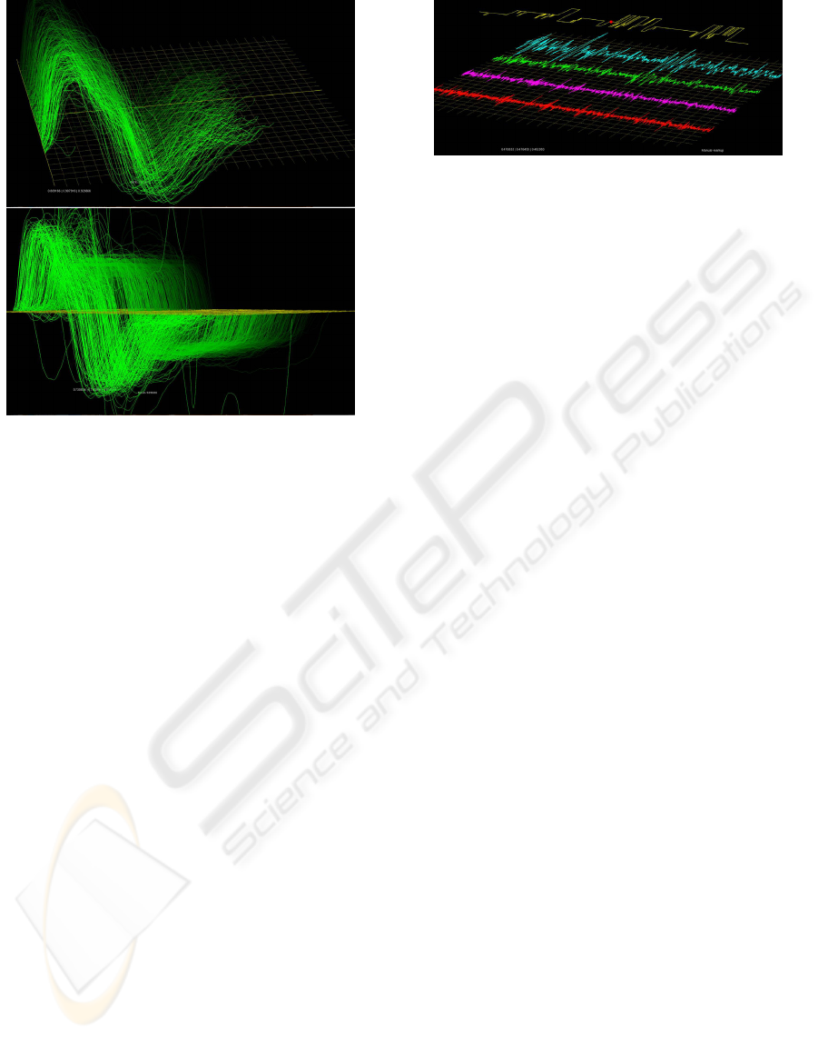
Figure 1: An animated sequence may be replayed with in-

dividual graphs separated in space to give the appearance of

‘depth’, or alternatively as a planar ‘cascade’. The bright-

ness of the graphs is modulated to add to the perception

of depth. Rotation and lighting effects allow one to move

around the objects dynamically to give advantageous views

of changing effects.

Traces may also be manually scrolled across the view-

ing space using mouse and key actions.

A contrasting animation effect is possible using

the X object speciﬁer. As with the free from graphs

(using the x speciﬁer) objects comprise an array of

], [y

], [z

] co-ordinate values, scaled and offset in

accordance with the header parameters. These objects

default to being simultaneously visible unless a fur-

ther instruction is included with the session. Alterna-

tively such a sequence of graphs may be played in an

animated sequence. An internal index counter deter-

mines the point in the graph sequence to be displayed,

and an index-range parameter determines how many

such graphs in the immediate vicinity of the current

position pointer are displayed simultaneously.

Sequence replay is modal. Figure 1 shows a snap-

shot from a series of 7000 graphs, with two different

views. In this viewing mode the graphs are placed in

sequence along the y-axis to create a sense of depth

that assists in visual interpretation of the data.

3.1.4 Mixing it all up

An important feature of S

is its ability to simul-

taneously handle a mix of object types. Surfaces, sta-

tic and animated graphs and curves may be combined

to reveal relationships within a set of complex signals,

and respective representations of these signals.

Figure 2: ‘Snapshot’ of animated polygraph data together

with a static graph of the full night’s sleep states (yellow,

offset above the polygraph traces). Planar static graphs and

animated traces, may be rotated and spun in the viewing

space, give useful perspective on the data traces.

Figure 3 shows an example of graphical objects de-

rived in relation to sleep analysis. The display corre-

sponds to the complete night’s data for one patient.

The entropy surface computed from the EEG/C3

channel, encapsulates all of the sleep state activity for

the night. The entropy surface cross-section at any

given point in time (represented by x-axis) is a rela-

tively precise, if not however convolved, measure of

signal source statistics over the corresponding sam-

ple periods. The peak values for the entropy, de-

ﬁned by the surface ridge (and graphed in red directly

above the ridge in the z-x plane), is graphed together

with the maximum entropy values for the EOC/LOC

(green). The latter is reﬂected in to the yx plane.

Plotting the maximum entropy values for C3 and

LOC against each results in the 3D trajectory (multi-

coloured). This trajectory is partitioned using planar

thresholds to divide the space into non-overlapping

volumes, and colour-coded accordingly; blue : awake

, red : REM sleep, green : S1, an NREM sleep state,

yellow : S2,S3,S4 NREM sleep states. S

then

encodes these coloured coded segments into numeri-

cally labeled states, displayed as the graph in yellow

below the surface.

4 CONCLUDING REMARKS

offers a novel approach to data visualisation.

As a interactive graphing and plotting tool, it accepts

data either as standard input or from appropriately for-

mated text ﬁles.

Graphical objects supported by the viewer include

surface arrays, static- and dynamic graphs of vari-

ous kinds, positional markers and combinations of

these. As many as 16,000 objects currently may

be simultaneously loaded for viewing. Surfaces are

limited to 2D regular array of ﬂoating point values

x,y

= s(x, y). Graphs in the zx or yx plane are pre-

scribed as lists of ﬂoating point values z

= f (x),

and y

= g(x), respectively. Trajectories may be pre-

scribed either by a 2D array, listing points y

GRAPP 2006 - COMPUTER GRAPHICS THEORY AND APPLICATIONS

382

Figure 3: The above includes static graphs of the entropy of

the EEG (red) and EOG (2 of green) channels. A 3D tra-

jectory is generated (above left) by plotting EEG and EOG

entropy series against one another. The trajectory is then

further partitioned by way of ‘invisible’ intersecting planes

and colour coded in respect of the volume associated sleep

states. The largely obscured graph (yellow) is generated as

a numerical encoding of the resultant states, and issues from

as standard output.

f(x) and z

== g(x) or independently of x, by list-

ing as a 3D array the coordinate points (x = f(i); y =

g(i); z = h(i), i =1, 2, 3 ...). Graphs are displayed

either as static or dynamic objects.

While many of the possible display modes have

been outlined here, it is not easy to convey in words

the full power of the dynamic and interactive as-

pects of the environment. The viewing experience,

as with other 3D graphical environments, is hugely

compelling in of itself, and S

is currently ﬁnd-

ing application in other research areas, outside of the

sleep studies.

Rather than being just another graphing tool, its

convenience and power to ﬂexibly present complex

data, combinations of static and animated graphs,

makes S

equally useful in technical presentation

settings. Though S

has stabilised considerably

since its inception, new features are being added at a

steady pace, in response to new visualisation require-

ments, thus augmenting its already considerable ver-

satility.

ACKNOWLEDGMENT

The author wishes to acknowledge that this research

work has been carried out with support from Fisher

and Paykel Healthcare (NZ) Ltd.

REFERENCES

Becker, R. A. and Chambers, J. M. (1981). S: A Language

and System for Data Analysis. AT&T Bell Laborato-

ries, Murray Hill, NJ, USA.

Char, B., Geddes, K., and Gonnet, G. (1983). The Maple

symbolic computation system. 17(3–4):31–42.

Clarke, A. and Kubrick, S. (1968). 2001: A Space Odyssey.

MGM, Polaris productions.

Ihaka, R. and Gentleman, R. (1996). R: A language for data

analysis and graphics. Journal of Computational and

Graphical Statistics, 5(3):299–314.

Kilgard, M. (1995). OpenGL: Let there be light! The X

Journal: Computing Technology with the X Window

System, 4(3):12.

Kilgard, M. J. (1996). OpenGL: Free OpenGL software.

The X Journal: Computing Technology with the X

Window System, 5(5):74.

Kochan, S. and Wood, P. (1990). UNIX Shell Programming.

pub-HAYDEN, revised edition.

Moler, C. B. (1980). MATLAB user’s guide. Technical re-

port, University of New Mexico. Dept. of Computer

Science. Describes use of Classic Matlab, the proto-

type for the expanded professional Matlab from The

MathWorks.

Schuster, H. and Just, W. (2005). Deterministic Chaos, an

introduction. Wiley-VCH, Berlin, revised edition.

Sleigh, J. W., Steyn-Ross, D. A., Steyn-Ross, M. L.,

Grant, C., and Ludbrook, G. (2004). Cortical entropy

changes with general anaesthesia: theory and experi-

ment. Physiological Measurement, 25, pp 921–934.

Steuer, R., Ebeling, W. B., and Titchener, M. R. (2001). Par-

tition based entropies. In Stochastics and Dynamics,

pp 45–61. World scientiﬁc.

Titchener, M. R., Gulliver, A., Nicolescu, R., Speidel, U.,

and Staiger, L. (2005). Deterministic information the-

ory. Fundamenta Informaticae, 64(1–4):443–461.

TOWARDS VISUAL-BANDWIDTH: GETTING CLOSE TO ONE’S EXPERIMENT DATA

383