A SYSTEMATIC APPROACH TO MULTIPLE DATASETS

VISUALIZATION OF SCALAR VOLUME DATA

Gaurav Khanduja and Bijaya B. Karki

Department of Computer Science, Louisiana State University, Baton Rouge, Louisiana, USA

Keywords: Multiple datasets visualization, Visualization application, Scalar data visualization, Isosurface, 3D textures,

Clipping.

Abstract: Many applications require simultaneous display of m

ultiple datasets, representing multiple samples, or

multiple conditions, or multiple simulation times, in the same visualization. Such multiple dataset

visualization (MDV) has to handle and render massive amounts of data concurrently. We analyze the

performance of two widely used techniques, namely, isosurface extraction and texture-based rendering for

visualization of multiple sets of the scalar volume data. Preliminary tests performed using up to 25 sets of

moderate-size (256

) data show that the calculated times for the generation and rendering of polygons

representing isosurface, and for the mapping of a series of textured slices increase non-uniformly with

increasing the number of individual datasets. Both techniques are found to no longer be interactive with the

frame-rates dropping below one for six or more datasets. To improve the MDV frame-rate, we propose a

scheme based on the combination of hardware-assisted texture mapping and general clipping. In essence, it

exploits the 3D surface texture mapping by rendering only the externally visible surfaces of all volume

datasets at a given instant, with dynamic clipping enabled to explore the interior of the data. The calculated

frame-rates remain above one and are substantially higher than those with the other two techniques.

1 INTRODUCTION

Visualization of three-dimensional scalar data has

been studied extensively over last two decades.

Tremendous challenge is often imposed by the size

of the volume data: Either the dataset is too massive

to exhaustively visualize or there are multiple

datasets to be visualized simultaneously. In this

paper, we have focused on the latter case, that is,

multiple datasets visualization (MDV) by which we

mean that more than one datasets of a given type are

concurrently rendered in the same visualization.

Although multiple datasets have previously been

visualized/analyzed in many occasions (Schulze and

Forberg, 2004; Crutcher et al., 1996; Abrams and

Shaffer, 1996), there exists a little work, if not at all,

towards addressing MDV in a systematic way.

We believe that there is no need to over

phasize on the importance of MDV. It is not

always possible to make an inference based on

single dataset so one needs to compare several

datasets in some effective way. So visualization

should be able to handle, multiple datasets at the

same time, representing multiple cases of interest so

that important relationships and differences among

these cases can be better understood.

Examples of multiple datasets, which require

sim

ultaneous visual analysis, are abundant. Here,

we consider 3D charge density distributions in real

material systems, which are investigated on routine

basis by parallel quantum mechanical simulations

(Codes, 2005). The resulting multiple charge density

datasets of interest may represent different samples,

or different temperatures or different pressures or

different simulation times. One might be interested

in comparing the charge distribution for different

(say four) types of vacancy defects in a given

crystal, say, Mg-, Si-, O1- and O2-defects in an

important Earth forming mineral MgSiO

perovskite.

Or the interest might be in investigating the effect of

pressure by displaying multiple datasets

corresponding to different pressure conditions (say

Mg-defect at eight different pressures) at the same

time. Or one might need to visualize together ten

different datasets as a function of temperature. Or, if

one is interested to look at outputs taken at different

times of simulation together, the number of datasets

can be arbitrarily large.

Khanduja G. and B. Karki B. (2006).

A SYSTEMATIC APPROACH TO MULTIPLE DATASETS VISUALIZATION OF SCALAR VOLUME DATA.

In Proceedings of the First International Conference on Computer Graphics Theory and Applications, pages 59-66

DOI: 10.5220/0001353200590066

 SciTePress

Two natural approaches to the multiple dataset

visualization appear to be a) an extension of the

standard visualization methods to handle multiple

datasets and b) a parallel processing (using multiple

CPUs and/or multiple display screens) of

visualization to permit real-time navigation through

multiple datasets. In this paper, we adopt the first

approach because it enables one to perform MDV

with easily available resources such as PC desktops.

A large number of 3D scalar visualization

techniques currently exist, and their performance is

often justified for single dataset visualization (SDV)

(Meibner et al. 2000). Common examples include

the isosurface extraction (Lorenson and Cline,

1987), raycasting (Levoy 1990), splatting

(Westover, 1990), shear-warp (Lacroute and Levoy,

1994) and texture mapping (Cabral et al, 1994).

Some of these approaches are considered here in the

context of the simultaneous visualization of multiple

datasets.

It is natural for one to expect that all standard

volume visualization techniques are equally

applicable to the case of visualization of multiple

datasets. However, this expectation is true to a great

extent but not entirely. MDV involves simultaneous

processing of more than one datasets. This means

that the visualization process should become slower

by a factor of N or higher for N number of datasets

in comparison with single dataset, due mainly to the

increased amount of data. The need for larger

memory space (which may eventually result in a

substantial swapping) and bigger display area

(which involves the processing of more pixels) can

further slow down the process. One other major

issue is that MDV is no longer guaranteed to be

interactive. Our preliminary performance tests show

that the SDV techniques studied here become

increasingly slow as the number of datasets

increases. Even for the data size of 256

, the frame-

rate is less than 1 for six or higher sets thereby

indicating the loss of interactivity in MDV.

Interactivity plays a crucial role in any volume

visualization and even more so in MDV because it

gives the user with immediate visual feedback. The

user often needs to repeat visualization process

several times, in part or full, to explore a given

dataset from various prospects. For instance, the user

might need to extract a series of isosurfaces

corresponding to different reference (or threshold)

scalar values. In the case of clipping, one might need

to examine many clipped views at different

locations, orientations and sizes. Even the direct

volume rendering, although no information is

thrown away, posses the difficulty of interpreting the

cloudy representation of the volume data. So the

extraction of a more complete information requires

several of interaction modes like navigation, changes

of transfer functions, region of interest mode,

rotation, scaling, and some more sophisticated

classification modes be supported in a given

visualization.

In this paper, we analyze the performance of two

standard volume visualization techniques, namely,

isosurface extraction and texture-based volume

rendering in the case of multiple datasets. Doing so

requires handling of massive amounts of data, which

introduces several issues related to memory,

resolution and interactivity. Our current focus is to

deal with the interactivity issue (by calculating the

frame-rate), which arises even in the case of multiple

datasets of moderate sizes, e.g., 256

. This size of

data is very common for today’s many scientific and

engineering applications. Also, this size can be

handled by the texture mapping support of the

today’s general-purpose graphics hardware. As an

effective solution to improving the interactivity, we

have adopted a MDV scheme based on 3D surface

texture mapping and general clipping. We limit the

maximum number of individual datasets to be

visualized together to 25 in this study.

2 RELATED WORK

Several visualization methods are available for

volumetric scalar datasets. Indirect methods extract

an intermediate geometric representation of the

surfaces from the volume data and render those

surfaces via conventional surface rendering

methods, e.g., isosurfaces (Lorenson and Cline,

1987). On the other hand, direct methods render the

data without generating an intermediate

representation and as such, they are more general

and flexible, e.g., texture-based rendering (Cabral et

al. 1994, Wilson et al. 1994). In addition to

supporting direct volume rendering, texture mapping

has also been used in conjunction with clipping

(Weiskopf et al. 2003). Both the strengths and

weaknesses of all these techniques have been

assessed in a wide variety of single dataset (Meibner

et al. 2000).

To the best of our knowledge, no systematic

analysis and practical evaluation of the current

volume visualization methods have yet been

reported in the case of multiple datasets. We choose

to examine the isosurface- and texture-based

visualization methods for MDV for several reasons:

First, the former is an indirect method whereas the

latter is a direct method. Second, the former is

software-based approach whereas the latter is the

hardware-assisted approach. Third, isosurface is so

widely used whereas texture mapping is faster than

the most volume visualization techniques.

GRAPP 2006 - COMPUTER GRAPHICS THEORY AND APPLICATIONS

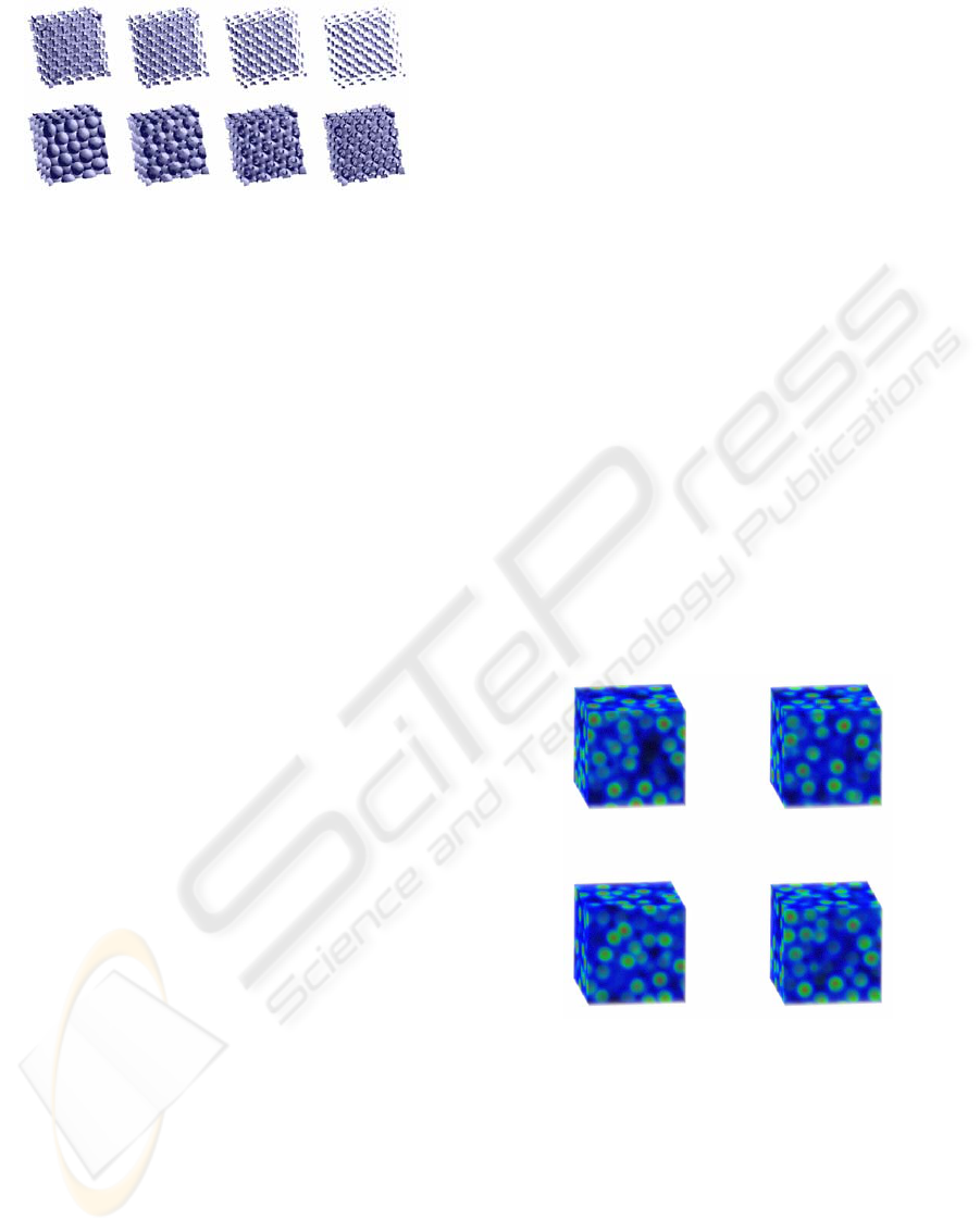
Figure 1: Isosurfaces for eight sets of the electronic charge

density data for MgO at different compressions

(compression increasing from the lower left to the upper

right). The structures represent the charge distribution

around O ion sites.

Due to recent advances of commodity graphics

hardware, texture-based rendering is able to achieve

acceptable frame-rates with high image quality

(Wilson et al. 1994; 2002; Weiler et al.2000; Cullip

and Newman, 2003). Clipping combined with

texture-based rendering can exploit advanced

fragment operations supported by graphics

hardware. For example, Van Gelder and Kim (1996)

have used clip planes. Techniques for volume

clipping with complex geometries, which are based

on the depth structure and voxelization of the clip

geometry and also involve subsequent shading of the

clipped surfaces, have been proposed (Weiskopf et

al. 2002; 2003). In the volume clipping based on

stencil tests, stencil buffer entries are set at only

those positions where the clip plane is covered by an

inside part of the clip geometry (Westermann and

Ertl, 1998). There are also techniques, which have

exploited isosurface clipping (Forguson, 1992) and

interactive clipping combined with dual-resolution

texture-based volume rendering (Khanduja and

Karki, 2005).

3 MDV WITH ISOSURFACE

An isosurface is the 3D surface representing the

locations of a constant scalar value within a volume.

Common approaches for generating isosurfaces

include the Marching Cubes algorithm for

generating isosurface polygons on a voxel-by-voxel

basis (Lorenson and Cline, 1987), the Dividing

Cubes approach of subdividing threshold voxels into

smaller cubes at the resolution of pixels (Cline et al,

1988), and raytracing with an analytic isosurface

intersection computation (Parker et al. 1998). We

use the Marching Cubes algorithm to extract

isosurfaces corresponding to a given threshold value

from multiple sets of data at the same time. The

essence of the algorithm remains the same for MDV:

It examines all voxels of each volume data (one by

one), and determines, from the arrangement of

vertex values above or below a threshold value, if

and how an isosurface would pass through these

elements. The algorithm thus processes one voxel at

a time, and generates its isosurface geometry

immediately before moving to the next voxel. Once

all the voxels of one volume data are processed and

the corresponding isosurface is extracted, the same

algorithm is repeated for each other volume data in a

given multiple set. We have visualized up to twenty-

five sets of 256

data using Marching Cubes

algorithm. Figure 1 shows MDV for the eight sets of

the simulated charge density of MgO as a function

of pressure.

4 MDV WITH 3D TEXTURE

RENDERING

The texture mapping approach uses 2D or 3D

textured data slices, combined with an appropriate

blending factor (Cabral et al. 1994; Wilson et al,

1994). In the case of 2D textures, three stacks of

slices, one for each major viewing axis, are stored

and one most parallel to the current viewing

direction is chosen. Hardware does bilinear

interpolation in a 2D texture only and opacity

changes with rotation. As such, image quality is best

Figure 2: Texture-based MDV of four sets of electronic

charge density distributions of MgO. The color and

opacity values for each pixel are based on the density

value associated with that pixel: A multiscale RGB color

mapping is used: B represents values from 0 to 0.05, G is

added to represent values up to 0.4 and then R is increased

and both B and G are decreased for higher values.

only when the slices are parallel to the view plane.

On the other hand, the 3D texture approach can

sample the data in all directions freely so the slices

can always be oriented perpendicular to the viewer's

line of sight. Image quality is independent of the

viewing direction. The intrinsic trilinear hardware

A SYSTEMATIC APPROACH TO MULTIPLE DATASETS VISUALIZATION OF SCALAR VOLUME DATA

interpolation allows us to perform supersampling,

i.e., to use an arbitrary number of slices with an

appropriate resampling on the slices. Only one

single 3D texture needs to be loaded thus requiring

one third of the memory, compared to the case of 2D

textures.

We apply the 3D texture-mapping hardware to

support MDV. The first step is to load the volume

data into a 3D texture; it involves simply reading a

set of images or shading data points. All datasets are

loaded one by one to generate multiple 3D textures.

The second step involves choosing the number of

slices perpendicular to the viewing direction for each

texture. The number of slices is often chosen to be

equal to the volume’s dimensions, measured in

texels. For instance, each dataset of 256

needs 256

slices. The third step is to use texture coordinate

generation to texture the slice properly with respect

to each 3D texture data. Finally, the textured slices

are rendered from back to front, towards the viewing

position, with appropriate blending performed at

each slice. In this study, OpenGL supported “over”

blending function is used. As the viewpoint and

direction of view change, one needs to recompute

the data slice positions and update the texture

transformation matrix as necessary.

5 INTERACTIVE MDV

APPROACH

We now adopt an approach by exploiting the

texture-mapping hardware and general clipping to

support a fast visualization of multiple sets of

volumetric scalar data. Similar approaches were

previously used to visualize a single dataset with

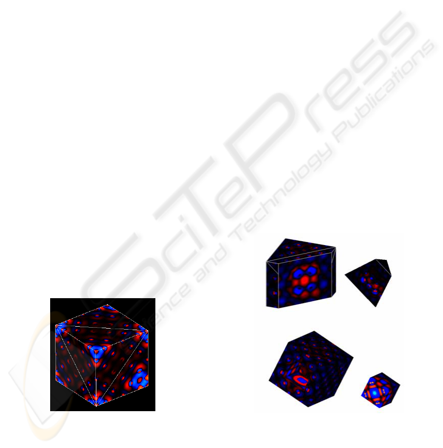
Figure 3: A 256

charge density data with the external

surfaces of the volume rendered using texture mapping.

Electrons are depleted from the bluish regions and

deposited in the reddish regions due to a vacancy defect in

MgO crystal.

interactive planar clipping and volume clipping via

per-fragment operations supported by graphics

hardware (van Gelder and Kim, 1996; Weiskopf et

al. 2003, 2003; Khanduja and Karki, 2005). They

involve rendering of all texels of the 3D textures

passing a given clip test, for instance, on average the

half of the total number of 256

texels are rendered.

Thus, the texture-based volume rendering with/out

clipping uses a large number of textured slices,

which becomes critical as the number of datasets to

be rendered concurrently increases.

5.1 External 3D Surface Rendering

Our texture-based MDV approach improves

interactivity by reducing the amount of texture

mapping. The basic idea is to restrict the rendering

of data to the external (visible) surfaces of the

volume instead of performing complete or nearly

complete 3D volume texture mapping. One place

where such surface rendering makes sense is the

visualization of the volume data by clipping. In the

case of clipping whether it uses a simple clip plane

or a more complex 3D clip geometry, one is always

interested to view the new surfaces that are exposed

(and hence are visible) to the user. For instance, one

can view scalar data on a cross-section of the

volume with a cutting plane. One defines a regular

grid on the clip plane and calculates data values on

this grid by interpolation of the original data and

Figure 4: Planar (upper two) and box (bottom two)

clipping. In the later case, inner (left) and outer (right)

portions of the volume are removed.

uses an appropriate color-map to make the data

visible. If this is the case and we are using 3D

texture-based rendering, then there is no need to

GRAPP 2006 - COMPUTER GRAPHICS THEORY AND APPLICATIONS

have texture mapped on all slices to cover the

complete volume.

Texture mapping is thus performed on only

external surfaces of the volume at a given instant

thereby restricting the rendering of the data only to

those visible surfaces. For instance, the simulated

charge density that considered here is confined to a

cubic volume. The 3D surface rendering of the

original volume can be done by simply extracting

and mapping textures on the six surfaces of the cube

front and back, left and right, and top and bottom

square faces), as shown in Figure 3. In effect, the

problem of 3D volume texture mapping is reduced

to the problem of 3D surface texture mapping, which

renders textured data on only those six surfaces.

Each square surface can be represented by two edge-

sharing triangles so that a total of 12 triangles thus

needed are used to implement the clipping operation,

which is described in the next Section. The 3D

surface rendering approach works only with the 3D

texture because it allows us to extract an arbitrary

textured-slice without requiring re-sampling of the

volume data. The polygon on which we want to map

a texture can intersect the volume at any location

and orientation. Texture mapping only requires the

vertices of this polygon, which are passed as texture

coordinates.

5.2 Clipping

Here we describe how clipping is combined with 3D

surface texture mapping. The purpose of clipping is

to find single or multiples surfaces cutting the

volume and then bound the intersecting surfaces in

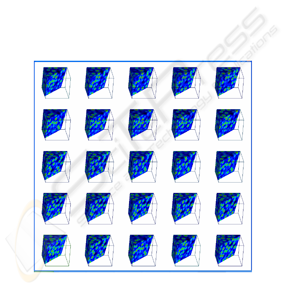
Figure 5: MDV of 25 sets of electronic charge density of liquid MgO (at different simulation times) using 3D surface

texture mapping combined with a planar clipping. One can see, for instance, how the positions of high density regions

(shown by green + red colors) change with time. A multiscale color map described in Figure 2 caption is used.

A SYSTEMATIC APPROACH TO MULTIPLE DATASETS VISUALIZATION OF SCALAR VOLUME DATA

the form of simple polygons. These polygons

determine the new set of externally visible surfaces

of the volume and the textured data is mapped only

on these polygons. Thus, only the surfaces defined

by a set of visible clipping polygons (single or

multiple) are rendered. Each clipping polygon is

tessellated in terms of triangles. During initial

rendering, the six planar surfaces of simulation box,

each represented in terms of two adjacent triangles

are rendered. During subsequent clipping process,

intersections of these 12 triangles with a given

object are calculated. If a triangle is intersected, it is

divided into two polygons that lie on either side of

the clip plane; and one of them is discarded.

Intersection points are used to define new polygons

to map textures. Every time the clip plane is

adjusted in 3D space, intersections of the original 12

triangles are determined to define polygons

(Stephenson and Christiansen, 1995), which bound

new visible surfaces

A planner clipping is demonstrated in Figure 4.

Every time a clip plane changes (rotates or translates

in space), new surfaces for texture mapping are

generated. We have also implemented a box-

clipping object, which is represented as a set of six

clipping planes. Visible surfaces are obtained by

repeating the same process, which is used in the case

of a single plane. The clip box can be rotated,

translated and resized. Figure 4 also shows the outer

and inner box clipping. Outer box clipping means

removing portion of 3D object that lie outside the

clipping box while the inner box clipping is just the

reverse of outer box clipping where the portion

outside the box is retained and portion inside the box

is removed.Figure 5 illustrates the simultaneous

visualization of 25 datasets.

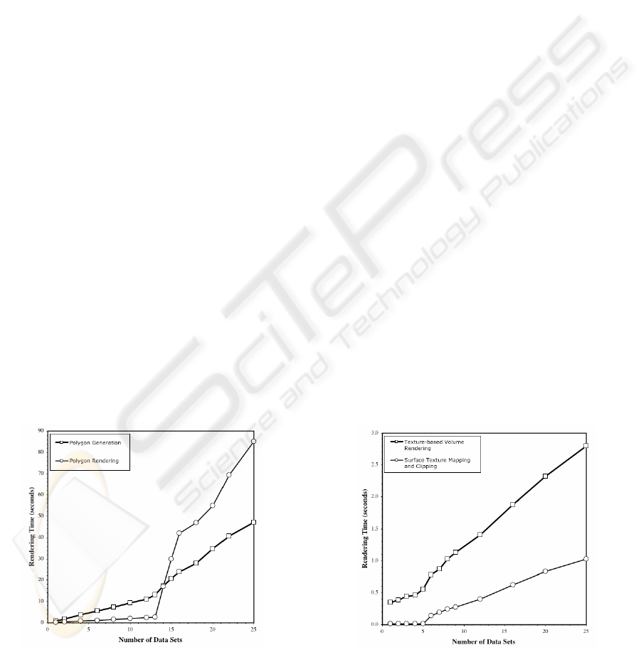
Figure 6: The calculated time as a function of the number

of datasets used in MDV. Squares represent the time for

generation of multiple lists for polygons representing

isosurfaces and circles represent the time for subsequent

rendering of polygons.

6 RESULTS AND DISCUSSION

We now present the performance measurements of

three MDV techniques described in the Sections 3, 4

and 5. The results are based on the 3D charge

density dataset, which was produced by parallel

quantum mechanical simulations for different

samples, conditions and time points. The size of

each dataset used is 256

, which represents today’s

common moderate-sized scalar volume data. The

rendering timings are calculated for single dataset

visualization (SDV) using the viewport of size 512

and for multiple dataset visualization (MDV) using

the viewport of size 1024

. A bigger viewport in

MDV provides bigger space for simultaneous

display of multiple datasets. Thus, the differences in

rendering speeds between SDV and MDV should

reflect the differences in the amounts of data to be

processed as well as the number of the pixels to be

displayed. The performance measurements have

been conducted on a Windows XP PC with 3.2 GHz

Pentium IV processor and 1 GB RAM. It uses an

NVidia GeForce FX 5200 graphics board with 128

MB graphics memory and 110 MB texture memory.

The implementation is based on C/C++, OpenGL

and GLUT.

Our analysis in the case of isosurface extraction

involves the calculation of the time for conversion of

the data into a set of polygons representing

isosurface and the time for subsequent rendering

with polygon rendering hardware (Figure 6). For

operations like rotation, translation and scaling, only

the rendering time is relevant. The calculated

rendering time is 0.16 seconds for SDV, and remains

below 3 seconds for MDV with up to 13 datasets. A

rapid increase starts when the number of datasets

increases reaches 14. This can be associated with the

Figure 7: The calculated rendering time as a function of

the number of datasets used in MDV. Squares represent

the time for the texture-based volume rendering and

circles represent the time for 3D surface texture mapping

combined with clipping.

GRAPP 2006 - COMPUTER GRAPHICS THEORY AND APPLICATIONS

limited memory so that more than 14 sets of

polygons representing isosurfaces cannot be stored

in the memory concurrently thereby involving

substantial memory swapping. The time for

multiple execution of Marching Cubes’ algorithm to

produce multiple sets of polygons increases more

rapidly with the increasing number of independent

datasets after 14 (Figure 6).

For the texture-based MDV, the calculated time

represents the time to map the textured data on a

series of slices (polygons) with an appropriate

blending enabled, i.e., to perform texture-based 3D

rendering (Figure 7). All 3D textures are assumed to

be already loaded/generated. The SDV rendering

time is 0.013 seconds whereas the MDV time is 1.12

and 2.81 seconds, respectively, for 9 and 25 datasets.

Note that the total number of slices to be rendered is

6400 for 25 datasets, compared to 256 slices for

single dataset. The number of independent texture

mappings becomes critical for texture-based MDV

as the number of datasets increases. Moreover, when

multiple sets of data are loaded as multiple textures,

all or most of the textures needed for generating

current view cannot be resident in the texture

memory at same time due to its limited size. So

swapping of the texture objects takes place between

the main memory and texture memory and the bus

bandwidth becomes a bottleneck. In our study, we

notice that up to five 3D textures can be concurrent

resident of the texture memory. This explains the

presence of a small abrupt increase in the calculated

time when the number of 3D textures (or

equivalently, 3D datasets) increases from 5 to 6.

Based on our preliminary tests discussed above,

the texture-based MDV shows a better performance

than the isosurface-based MDV (Table I).

However, the frame-rates are low for the both

approaches in the context of interactivity. Even for

the moderate datasize of 256

considered here, the

frame-rate drops below 1 for six or higher number of

datasets. In the case of isosurface, if one is interested

to change the threshold isovalue to get a new set of

isosurfaces during MDV process, the processing

time becomes much longer.

We have also calculated the rendering time for

the proposed MDV approach, which uses 3D surface

texture mapping combined with a planar or box

clipping. The MDV time is very small for datasets

up to 5 and then it increases suddenly for 6 sets and

thereafter increases gradually as the number of

datasets increases (Figure 7). The rapid increase can

again be associated with the limited memory as

discussed earlier. The results show that the proposed

MDV improves the frame-rate substantially (Table

I). First of all, the frame-rate remains above one.

Second, it is larger by a factor of 3 than that of the

3D volume texture rendering for MDV with 6 to 25

sets of data. This is consistent with the fact that the

number of the slices or polygons rendered is

dramatically reduced in the texture-based surface

rendering, compared to that in the corresponding

volume rendering. For simultaneous visualization of

25 datasets, each of size 256

, the 3D surface texture

mapping needs a couple of hundreds of polygons,

compared to 6,000 slices (or more polygons)

required by the 3D volume texture mapping. Third,

the differences with respect to the isosurface-based

MDV are even bigger (Table I).

7 CONCLUSIONS

In this paper, we have presented a systematic

analysis of the multiple dataset visualization (MDV).

Many applications require datasets to be grouped

and analyzed together based on certain criteria such

as samples, conditions, and time-points. In

particular, we have performed MDV using two well-

known techniques, which are based on isosurface-

extraction and hardware-assisted texture mapping.

Our results have shown that the both techniques

yield low frame-rates when six or more sets of

moderate-sized (256

) data are visualized

concurrently. Besides the issues related to the larger

memory requirements and limited display sizes, one

important challenge is to make MDV interactive.

We have proposed an interactive MDV approach in

which the 3D surface texture mapping and clipping

are exploited. The basic idea is to avoid the

rendering of all the textured slices to cover complete

or nearly complete volume data by restricting texture

mapping onto the only externally visible surfaces of

each volume data. The interior of the volume is then

explored by exposing (and subsequently rendering)

new surfaces with dynamic manipulation of some

form of clipping such as a planar or box clipping

enabled. For as many as 25 sets of 256

data

visualized concurrently, our approach yields more

than one frame per second, compared to much less

than one frame per second with isosurfacing and 3D

volume texture mapping. Our scheme is expected to

be an effective MDV tool since it exploits the

essence of general clipping to uncover important,

otherwise hidden details of volume data sets to the

extent which is often not feasible with other

techniques. At the same time, it also benefits from

the increasing processing power and flexibility of

graphics processing unit.

A SYSTEMATIC APPROACH TO MULTIPLE DATASETS VISUALIZATION OF SCALAR VOLUME DATA

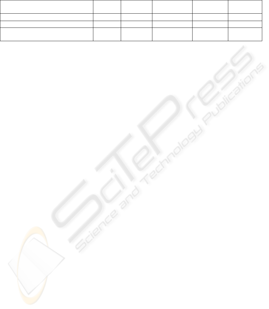
Table 1: Comparison of the calculated frame-rates (number of frames per second, fps) between three different methods for

single dataset visualization (SDV), and multiple dataset visualization (MDV) with different number of datasets.

We plan to implement more complex clip

geometries and extend the performance analyses to

multiple sets of 512

or larger data.

ACKNOWLEDGMENTS

This work was supported by NSF Career (EAR 0347204)

and ITR (ATM 0426601) grants.

REFERENCES

Abrams, M. and Shaffer, C., 1996. www.sv.vt.edu/future

/ari/white/abrams_shaffer.html

Cabral, B., Cam, N. and Foran, J, 1994. Accelerated

volume rendering and tomographic reconstruction

using texture-mapping hardware. Proc. 1994 Symp.

Volume Visualization. 91-98.

Cline, H., Lorensen, W., Ludke S., Crawford, C., and

Teter, B., 1988. Two algorithms for three dimensional

reconstruction of tomographs, Medical Physics. Vol.

15.

Codes, 2005. Electronic calculation packages: PWScf

(www.pwscf.org) and VASP (cms.mpi.univie.ac.at

/vasp).

Crutcher, R.M., Baker, M.P., Baxter, H., Pixton, J. and

Ravlin, H., 1996. Astronomical Data Analysis

Software and Systems V, ASP Conference Series, Vol.

101.

Cullip, T.J. and Newman, U., 1993. Accelerating volume

reconstruction with 3d texture hardware. Technical

Report TR93-027, University of North Carolina,

Chapel Hill, N. C.

Van Gelder, A., and Kim, K., 1996, Direct volume

rendering with shading via three-dimensional textures.

Proc. 1996 Symp. Vol. Visualization, 23-30.

Khanduja, G. and Karki, B. B. 2005. Visualization of 3D

scientific datasets based on interactive clipping.

WSCG Int. Conf. Computer Graphics, Visualization

and Computer Vision, SBN 80-903100-9-5, 33-36.

Lacroute, P. and Levoy, M., 1994. Fast volume rendering

using a shear-warp factorization of the viewing

transformation. Proc. SIGGRAPH’94, 451-458.

Levoy, M., 1990. Efficient ray tracing of volume data,

ACM Trans. Comp. Graphics., 8, 245-261.

Lorensen, W.E. and Cline H.E., 1987. Marching Cubes: a

high-resolution 3D surface reconstruction algorithm.

Computer Graphics Proc. SIGGRAPH, 21, 163-169.

Meibner, M., Huang, J., Bartz, D., Mueller, K. and

Crawfis, R., 2000. A practical evaluation of popular

volume rendering algorithms, Proc. of the 2000 IEEE

Symps. Volume Visualization, 81-90.

Parker S., Shirley, P., Livnat, Y. Hansen, C., and Sloan,

P., 1998, Interactive ray tracing for isosurface

rendering, Proc. Visualization ‘98, 233-238.

Stephenson, M. B. and Christiansen, H. N., 1975. A

polyhedron clipping and capping algorithm and a

display system for three dimensional finite element

models. ACM SIGGRAPH.

Schulze, J.P., and Forsberg, A.S., 2004. User-friendly

volume data set exploration in the Cave,

www.cs.brown.edu/people/schulze/vis04-contest.

Weiler, M., Westermann, R., Hansen, C., Zimmerman, K.,

and Ertl, T., 2000.. Level-of-detail volume rendering

via 3D textures. In Proceedings of IEEE Volume

Visualization 2000.

Weiskopf D., Engel, K., and Ertl, T., 2003. Interactive

Clipping Techniques for Texture-Based Volume

Visualization and Volume Shading. IEEE

Transactions on Visualization and Computer Graphic,

9, 298-312.

Weiskopf, D., Engle, K. and Ertl, T., 2002. Volume

clipping via per-fragment operations in texture-based

volume visualization, IEEE Visualization Proc. 2002,

93-100.

Westermann, R. and Ertl, T., 1998, Efficiently using

graphics hardware in Volume Rendering Applications.

SIGGRAPH 1998 Proc., 169-179.

Westover, L., 1990. Footprint evaluation for volume

rendering. SIGGRAPH’90, 367-376.

Wilson B., Ma, K. and McCormick, P.S., 2002. A

hardware-assisted hybrid rendering technique for

interactive volume visualization. Proc Vol.

Visualization and Graphics Symp. 2002.

Forguson, 1992. Visual Kinematics, Inc. (Mountain View,

CA USA), FOCUS User Manual, Release 1.2.

Wilson, O., van Gelder, A. and Wilhems, J., 1994. Direct

volume rendering via 3d textures. Technical Report

UCSC-CRL-94-19, Jack Baskin School of Eng., Univ

of California at Santa Cruz.

Methods SDV

MDV

4 datasets

MDV

9 datasets

MDV

16 datasets

MDV

25 datasets

Isosurface: Polygon rendering 5.02 1.221 0.556 0.024 0.012

Texture-based volume rendering 7.61 2.153 0.878 0.532 0.357

Clipping with surface texture

mapping

>75 ~75 3.597 1.611 1.002

GRAPP 2006 - COMPUTER GRAPHICS THEORY AND APPLICATIONS