DATA PROCESSING AND COMPACT REPRESENTATION OF

MEASURED ISOTROPIC SPECTRAL BRDF

Huiying Xu

Department of Computer Sciences, Purdue University, West Lafayette, Indiana 47907, USA

Keywords: BRDF, Data processing, Representation.

Abstract: This paper presents the methods for both data processing and compact representation of measured isotropic

spectral BRDF. For the data processing, we develop a numerical method for filtering the noises, re-sampling

the data from non-uniform sampling to uniform sampling, and interpolation. For the compact representation,

we propose a method to represent the spectral BRDF in both the spectral and spatial domains. In spectral

domain, for each pair of the incident and outgoing directions, we represent the spectral BRDF with Fourier

coefficients. In spatial domain, for all the outgoing directions of a given incident direction, we represent the

same-order Fourier coefficients either directly using a linear combination of spherical harmonics or a linear

combination of spherical harmonics and a Gaussian, depending on their angular dependencies. Three

Gaussian expressions are presented. Numerical studies are given for a measured isotropic spectral BRDF.

1 INTRODUCTION

Characterizing light reflection from object surfaces

is essential in many areas, such as computer graphics

and visualization, image analysis, remote sensing,

medical imaging, confocal microscopy imaging,

computational simulation, nondestructive inspection,

and etc. The surface light reflections are generally

described by a bi-directional reflection distribution

function (BRDF)

(,,)

(,, , ,)

(,,)cos

ooo

iioo

iii i i

θϕλ

ρθ ϕ θ ϕ λ

θϕλ θ

Ω

, (1)

which is the ratio of the reflected radiance

dL in

direction

(, )

to the incident irradiance

cos

iii

Ω in solid angle sin

iiii

ddd

θϕ

Ω= (Figure

1), and

is the wavelength. The incident (or

lighting) and outgoing (or viewing) directions are

specified respectively using the angle pairs

(, )

and

(, )

Some analytic models have been developed to

describe surface reflection behavior. However, the

current analytic models were developed based on

various assumptions so that they are not applicable

for all kinds of surfaces. Alternatively, one may

obtain the raw data of BRDFs from the experimental

measurements. However, there are some problems

with the raw data. First, the data has unavoidably

involved the noises so that the data cannot be

directly used. Second, we cannot measure the raw

data for arbitrary pair of incident and outgoing

directions, so we need a method to accurately

interpolate the unmeasured pairs from all the

measured pairs. Third, the measured raw data is

often non-uniformly sampled. However, in some

cases the uniformly sampled data is necessary for

practical application. Fourth, since a spectral BRDF

is a five dimensional function, the storage of raw

data unavoidably occupies a huge space.

Figure 1: The geometry and notations of BRDF definition.

In this paper, we present the methods for both

the data processing and compact representation. For

the data processing, we developed a method to filter

the noises involved in the raw data, resample the

data, and interpolate it for the unmeasured pairs of

407

Xu H. (2006).

DATA PROCESSING AND COMPACT REPRESENTATION OF MEASURED ISOTROPIC SPECTRAL BRDF.

In Proceedings of the First International Conference on Computer Graphics Theory and Applications, pages 407-414

DOI: 10.5220/0001352404070414

 SciTePress

incident and outgoing directions. For the compact

representation, we proposed a method to represent

the spectral BRDF. In this method, for each pair of

the incident and outgoing directions, we represent a

BRDF with the Fourier coefficients. For all the

outgoing directions of a given incident direction, we

represent the same-order Fourier coefficients either

directly using a linear combination of spherical

harmonics or using a linear combination of spherical

harmonics and a Gaussian, based on their angular

dependencies. The reconstruction of spectral BRDF

from representation just reverses this process.

This paper is organized as the follows. Section 2

reviews the background. Section 3 elaborates the

data processing method. Section 4 describes the

representation method. Section 5 presents the

numerical studies. Section 6 gives the conclusions

and future work.

2 BACKGROUND

Current analytic models commonly decompose the

entire reflection into the diffuse and specular

components. The diffuse component is typically

assumed to be a Lambertian, but the specular

component varies among models. A simple approach

describes the specular component with the empirical

functions (Phong, 1975; Strauss, 1990). More

accurate models were developed from physically

based approaches. One physically based approach

uses Kirchoff theory with the tangent plane

approximation (Beckmann, 1963). He et al. (1991)

used this approach to model complex effects

including light polarization, surface masking and

shadowing, and subsurface scattering. Another

approach is based on the Torrance-Sparrow

microfacet model of surfaces (Torrance, 1967). This

model assumes that a rough surface is comprised of

many V-shaped planar, perfectly smooth, and

isotropic microfacets. The specular component is

expressed as a product of the Fresnel coefficient, the

masking and shadowing factor, and the surface

orientation probability, as presented in the Blinn-

Cook-Torrance model (Blinn, 1977; Cook, 1982).

An early measurement of BRDFs used gonio-

reflectometer (Murray-Coleman, 1990). However,

the equipment is very expensive, and the

measurement takes very long time. Ward (1992)

introduced a novel device called imaging gonio-

reflectometer. This system uses a half-silvered

hemispherical mirror to collect the light from the

sample surface and reflect it back into a CCD

camera with a fisheye lens. This device is

inexpensive and the measurement is relatively faster.

Dana et al. (1999) developed a simple system to

measure bidirectional texture functions and BRDFs.

Marschner et al. (1999, 2000) constructed a simple

and rapid system to measure isotropic surfaces with

spherical geometry. Matusik et al. (2003a, 2003b)

developed a similar device and measured densely

sampled BRDF data for different materials.

Recently, Sun et al. (2005) measured some spectral

BRDFs by the sample-rotated method. In which, the

spectrum is captured by a PR-650 SpectraScan

colorimeter. During the entire measurement, the

colorimeter is fixed. Instead, the sample is rotated

very often and the light source is relocated several

times for all sampled incident and outgoing

directions.

To save the storage space, it is desirable to

represent the BRDF with fewer parameters. There

are three popular representation methods. The first is

representing a BRDF in terms of an empirical or

physical model (Ward, 1992; Lafortune, 1997). This

method is compact, but inaccurate. The second is

representing a BRDF with a linear combination of a

set of basis functions, such as spherical harmonics

(Carbal, 1987; Sillion, 1991), Zernike polynomials

(Koenderink, 1998), and wavelets (Schröder, 1995;

Lalonde, 1997). The third is factoring a high-

dimensional BRDF into a sum of low-dimensional

functions (Fournier, 1995; DeYong, 1997). The

second and third methods have the same problem:

there exists a trade-off between the accuracy and

compactness. For example, given a BRDF with the

sensitive angular dependency, the larger number of

coefficients is used, the more accurate the

representation, but the less compact.

Most of the previous measurements and

representations focused on the non-spectral BRDF

(such as RGB-based). However, spectral BRDF

offers the better commitment for faithful image

rendering and analysis. Therefore, we need to

develop the correspondent methods for the noises

filtering, data re-sampling, data interpolation, and

compact representation of measured spectral BRDF.

All of these considerations ignite the current work.

3 DATA PROCESSING METHOD

The errors involved in the measurement of spectral

BRDF are diversified. First, for different outgoing

directions, the sample surface viewed by the

colorimeter is different. The larger is the angle

between the surface normal and outgoing direction,

the larger is the area. Since the sample surface is not

GRAPP 2006 - COMPUTER GRAPHICS THEORY AND APPLICATIONS

408

()

t t

()F

()

t ()F

()

tkT

−

∑

()

strictly smooth and isotropic, the measured spectra

must involve some errors. Second, since the sample,

light source, and colorimeter are rotated or located

manually, this can result in another kind of errors.

Third, the unstable intensity of light source can also

be a source of errors.

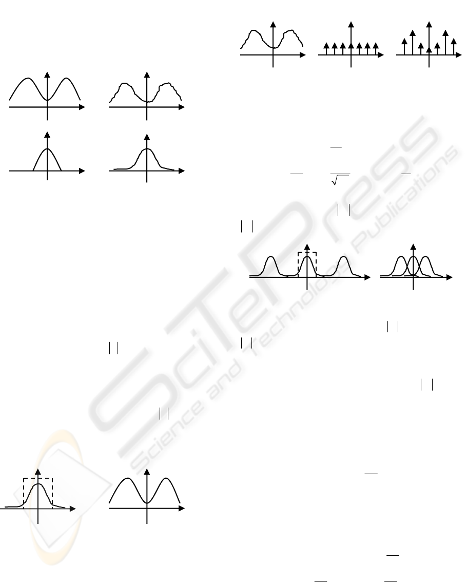
(a) (b)

Figure 2: Fourier transformations of ()

t without noises

(a) and with noises (b).

Generally, the contribution of experimental

errors to the measured data oscillates quickly

between the positive and negative effects. Therefore,

we can regard them as the noises that are dominated

by the high frequency components. Consider one-

dimensional case, Fourier transformations of

()

with and without the noises are shown in Figure 2.

In the subfigure (a), we can find a cut-off frequency

so that () 0F

= for

. However, in the

subfigure (b), it is difficult to find such a cut-off

frequency since the noises contribute wide high

frequency components to the spectrum

()F

Therefore, to filter the noises, we can cut off the

high frequency components with

> , and

perform inverse Fourier transformation to get the

clean raw data, as shown in Figure 3.

Figure 3: Inverse Fourier transformations for noises

removing.

Given the one-dimensional function

()

t , the

uniformly sampled data

()

with the period

can be expressed as (Glassner, 1995)

() () ( )

nT f t t kT

=−

∑

. (2)

The sampling process is shown in Figure 4.

Figure 4: Illustration of uniform data sampling.

Using the property of convolution, Fourier

transformation of the sampled data

()

nT is given

as (Glassner, 1995)

() ( )

GFk

ωω

=−

∑

, (3)

where

= ,

= , and

= .

()G

shown in Figure 5. We can see that, copies of

()F

overlap just a little for

> , and quite a lot for

< .

(a) (b)

Figure 5: Illustration of

()G

for

> (a) and

< (b).

To filter the noises from

()

t , we need to sample

the raw data with the period

so that

> .

Then we can multiply

()G

with a box spectrum

()

, as dotted line shown in Figure 5(a). Finally

we perform the inverse Fourier transformation to

obtain the filtered

()

t . The one-dimensional

expression is given as (Glassner, 1995)

() ( )sinc ( )

tgnT tnT

⎡⎤

=−

⎢⎥

⎣⎦

∑

. (4)

The isotropic BRDF can be described by a four-

dimensional function with the parameters

and

. Following Eqs. (2-4), the BRDF for each

component of wavelength is given as

(, , ) [,,]sinc[ ( )]

sinc[ ( )]sinc[ ( )]

ioo i

mn l

mnl mT

nT lT

λλ

ρθθϕ θ

θϕ

ππ

=−

⋅− −

∑∑∑

(5)

where

T ,

T and

T are the sampled periods for

and

, respectively,

[,,]

mnl

is the uniformly

DATA PROCESSING AND COMPACT REPRESENTATION OF MEASURED ISOTROPIC SPECTRAL BRDF

409

sampled data for the grid point (

= ), and

= ,

= , and

= .

Although the raw data of measured spectral

BRDF is non-uniformly sampled and densely

distributed, we can obtain the optimal solution

[,,]

mnl

by solving the linear least squares problem

min [ , , ]sinc[ ( )]

sinc[ ( )sinc[ ( )

raw i

mn l

mnl mT

mT mT

ρθ

θϕ

ππ

−−

⋅− −

∑∑∑

, (6)

with the constraint

[,,] 0gmnl

≥ . This constraint

comes from the property that the reflectance is non-

negative. We can implement the non-negative least

squares (NNLS) algorithm (Lawson, 1995) to solve

this constrained linear least squares problem.

For the outgoing directions perpendicular to the

sample surface, the BRDF has the property:

(,0,0) (,0,) (,0, )

ii i

TlT

ρθ ρθ ρθ

==⋅⋅⋅=

. (7)

In addition, the isotropic BRDF has the property:

(0, ,0, ) (0, , , ) (0, , , )

oo o

TlT

θλρθ λ ρθ λ

==⋅⋅⋅= . (8)

Therefore, we renormalize the matrix in Eq. (6) so

that the optimal solution still satisfies these

properties. Assume that

x= for the following

linear least squares problem

11 12 13 1 1

21 22 23 2 2

31 32 33 3 3

min

aaa x b

⎛⎞⎛⎞⎛⎞

⎜⎟⎜⎟⎜⎟

−

⎜⎟⎜⎟⎜⎟

⎝⎠⎝⎠⎝⎠

, (8)

the matrix can be renormalized so that the linear

least squares problem becomes

11 12 13 1

21 22 23 2

31 32 33 3

min

aaa b

⎛⎞⎛⎞

⎛⎞

⎜⎟⎜⎟

+−

⎜⎟

⎜⎟⎜⎟

⎝⎠

⎜⎟⎜⎟

⎝⎠⎝⎠

. (9)

For the outgoing directions far away from the

highlights, the BRDF varies smoothly and gradually.

Hence, the raw data is usually captured sparsely.

However, the sparse data can result in the failure of

solving Eq. (6). To solve this problem, we introduce

the following linear relations into the linear least

squares problem

[ 1,,] 2 [,,] [ 1,,] 0

[, 1,]2 [,,] [, 1,] 0

[,, 1]2 [,,] [,, 1] 0

gm nl gmnl gm nl

gmn l gmnl gmn l

gmnl gmnl gmnl

λλλ

−− ++=

−− + +=

. (10)

It is obvious that the optimal solution is

uniformly sampled. To interpolate the BRDF for any

unmeasured pair of incident and outdoing directions,

we just need to follow Eq. (5).

4 REPRESENTATION METHOD

Our representation method consists of two stages. In

the first, we represent the spectral BRDF in the

spectral domain. In the second, we represent the

Fourier coefficients in spatial domain.

4.1 Spectral Domain

For each pair of incident and outgoing directions, a

spectral BRDF is a spectrum. Therefore, we perform

Fourier transformation to it and represent it with

Fourier coefficients. The expression is given as

min

(, , ,) (, , )

2( )

(, , )cos

2( )

(, , )sin

ioo ioo

kioo

ρθθϕλ θθϕ

πλλ

θθϕ

πλλ

θθϕ

⎧

−

⎡

⎤

⎨

⎢

⎥

∆

⎣

⎦

⎩

⎫

−

⎡⎤

⎬

⎢⎥

∆

⎣⎦

⎭

∑

(11)

where

max min

λλ

∆

=− is the visible range, and

max

min

max

min

(, , ) (, , ,),

2( )

cos , 0,1, ,

(, , ) (, , ,),

2( )

sin , 1,2, ,

kioo ioo

θθϕ λρθθ ϕ λ

πλλ

θθϕ λρθθ ϕ λ

πλλ

∆

−

⎡⎤

⋅

=∞

⎢⎥

∆

⎣⎦

∆

−

⎡⎤

⋅

=∞

⎢⎥

∆

⎣⎦

∫

(12)

4.2 Spatial Domain

For all the outgoing directions of a given incident

direction, we represent the same-order Fourier

coefficients. If these coefficients have insensitive

angular dependencies on the outgoing directions, we

represent them directly using a linear combination of

spherical harmonics. Otherwise, we decompose

them into a smooth background and a sharp lobe.

Since the smooth background is dominated by the

low-frequency components, we can represent them

efficiently using a linear combination of low-level

spherical harmonics. The sharp lobe is dominated by

the high-frequency components, so we represent it

using a Gaussian. The decomposition is shown in

Figure 6. For the kth Fourier coefficients, the

representation is given as

,(, )

() (, ) (, , )

ilmo o kio o

klm

lml

AY G

θϕ θθϕ

==−

∑∑

. (13)

Here the first term represents the smooth

background,

(, )

lm o o

is the spherical harmonic

with the level (

l ,

the maximum level, and

GRAPP 2006 - COMPUTER GRAPHICS THEORY AND APPLICATIONS

410

,(, )

()

klm

the coefficients. The second term

(, , )

kioo

θϕ

represents the sharp lobe, and it is a

Gaussian.

(a)

(b)

(c)

Figure 6: Decomposition of the same-order Fourier

coefficients (a) into a smooth background (b) and a sharp

lobe (c).

In this paper, we tried three Gaussians for the

representation of the sharp lobe. The first is given as

(, , ) exp[ (, , ) ]

kioo k kioo k

Gp b

θθϕ α θθϕ

=− , (14)

where

and

b specify the height and width of the

sharp lobe, and

(, , )

kioo

θθϕ

is the angle between the

outgoing direction

(, )

and the direction of the

peak of sharp lobe. For the isotropic spectral BRDF,

the direction of the peak of sharp lobe is a function

. The second is generated from the empirical

model (Ward, 1992)

( , , ) exp[ tan ( , , ) ]

kioo k kioo k

Gp b

θθϕ α θθϕ

=− , (15)

and the third from the physically based model (Sun,

2004)

( , , ) exp[ tan ( , , ) ]

kioo k kioo k

Gp b

θθϕ α θθ ϕ

=− . (16)

The decomposition of Fourier coefficients into a

smooth background and a sharp lobe is a key point

for this representation method. To achieve this, we

need to obtain the critical angle first. Then, for all

the outgoing directions with the angles from the

peak of the sharp lobe are larger than the critical

angle, we treat the Fourier coefficients as the smooth

background. We can use the regression analysis (or

linear least squares) to determine the coefficients

,(, )

()

klm

. Finally, we extract the smooth

background from the Fourier coefficients, and use

the regression analysis (or linear least squares) to

determine the coefficients

p and

b .

Finding the critical angle is a little tricky since

we cannot directly obtain it from the raw data. In

this paper, we first evaluate the range of critical

angle from the raw data. Then we uniformly sample

the range with a reasonable interval. For each

sampled angle, we take it as the critical angle and

use it for the decomposition. Correspondently we

calculate the relative error between the raw data and

the representation. Finally we select the sampled

angle with the least relative error as the real critical

angle.

5 NUMERICAL STUDIES

In this paper, the raw data of spectral BRDF is

measured from a sample “ME01_AmberGlass”. The

data is non-uniformly sampled for the incident and

outgoing directions in terms of the geometry of

BRDF, and has the noises involved. Furthermore,

the data is sparsely distributed around some pairs of

incident and outgoing directions, while it is densely

distributed around some other directions.

5.1 Data Processing

Following Eqs. (5-10), we obtain the uniformly

sampled and noises-filtered spectral BRDF data. For

different incident angle

, the spectral BRDF at

550nm

for different outgoing directions is

shown in Figure 7. In this paper,

=−

stands for

the outgoing direction

(,0)

° , and

= for

DATA PROCESSING AND COMPACT REPRESENTATION OF MEASURED ISOTROPIC SPECTRAL BRDF

411

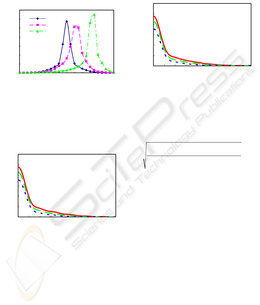
( ,180 )

° . We can see that the BRDF shows apparent

off-specular reflection for

15 ,45

=° °. Moreover,

the BRDF shows higher peak for normal incidence,

and for the incidence close to the grazing direction.

0.00

0.20

0.40

0.60

0.80

1.00

1.20

1.40

-90-75-60-45-30-150 153045607590

Theta (degree)

BRDF

line 1

line 2

line 3

Figure 7: Spectral BRDF at

550nm

for 0

=° (line 1),

=° (line 2), and 45

=° (line 3).

Following Eq. (5), we interpolate the spectral

BRDF for the unmeasured pairs of incident and

outgoing directions. By converting the spectra into

the RGB color components, the BRDF for normal

incidence is shown in Figure 8.

0 102030405060708090

Theta (degree)

BRDF (RGB)

Figure 8: Interpolated BRDF for normal incidence.

From Figure 8, we can see some oscillations for

10 60

°< < °. This phenomenon is commonly called

the ring effect. It may come from two reasons. One

is caused from the introduction of linear relations, as

shown in Eq. (10), and another from the inherit ring

effect of Eq. (5) (Glassner, 1995). To remove the

ring effect, we multiply a window function

(,,)wmnl

to the right term of Eq. (5),

(,,) cos[2( )]

cos[2( )]cos[2( )]

wmnl mT

nT lT

θϕ

=−

⋅− −

. (17)

In calculation, we always take

(,,) 0wmnl

for some cases. The interpolated BRDF

with the ring effect removed is shown in Figure 9.

0 102030405060708090

Theta (degree)

BRDF (RGB)

Figure 9: Interpolated BRDF with the ring effect removed

for normal incidence.

5.2 Representation

The accuracy of a representation method can be

evaluated in terms of the relative error between the

reconstructed spectral BRDF and the original one

(, , ) (, , )

(, , )

reconstr i o o orig i o o

orig i o o

λθ ϕ

ρ θθϕ ρ θθϕ

ρθθϕ

⎡

⎤

−

⎣

⎦

⎡⎤

⎣⎦

∑∑∑

,(18)

where

(, , )

reconstr i o o

θθϕ

and (, , )

orig i o o

θθϕ

are the

reconstructed and original spectral BRDFs,

respectively.

For the re-sampled and noises-filtered data, we

represent the spectral BRDF for each pair of incident

and outgoing directions with 19 Fourier coefficients,

while the original data size is 101. Since the spectral

BRDF is sensitively angular dependent, the same-

order Fourier coefficients of each sampled incident

direction is also highly angular dependent. We have

to decompose the Fourier coefficients into a smooth

background and a sharp lobe, and represent them

respectively. For normal incidence, Figure 9 shows

the comparisons between the original data and the

ones reconstructed from the representations at

550nm

. Here, the line “orig” stands for the

original data, the line “rep 1” for the representation

using Eq. (14), the line “rep 2” for that using Eq.

(15), and the line “rep 3” for that using Eq. (16).

For

, as shown in Figure 9(a), the

representation error for the representation using

either Eq. (14) or Eq. (15) is 14.3%, and that using

Eq. (16) is 11.5%. From Figure 9(a), we can see that

the representation error mainly comes from the

GRAPP 2006 - COMPUTER GRAPHICS THEORY AND APPLICATIONS

412

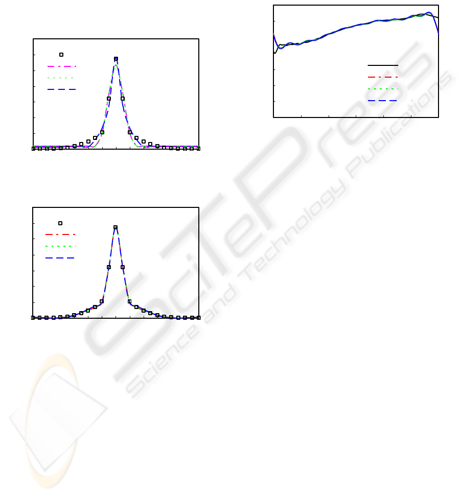
representation for the smooth background; this is

due to the fact that the low-level spherical harmonics

cannot represent the high-frequency components

completely. Moreover, we can see that the

representation using Eq. (16) matches the sharp lobe

of the original data better than the representations

using Eq. (14) and Eq. (15). This fact indicates that

the physical model (Sun, 2004) might match the

original data better than the empirical model (Ward,

1992).

0.2

0.4

0.6

0.8

1.2

1.4

-90 -75 -60 -45 -30 -15 0 15 30 45 60 75 90

Theta (degree)

BRDF

orig

rep 1

rep 2

rep 3

(a)

0.2

0.4

0.6

0.8

1.2

1.4

-90-75-60-45-30-150 153045607590

Theta (degree)

BRDF

orig

rep 1

rep 2

rep 3

(b)

Figure 10: Comparisons between the original data and the

representations for normal incidence.

For 4

= , as shown in Figure 9(b), the

representation error for using each of Eqs. (14-16) is

lower than 4.5%. Here, the total number of

coefficients used for representation is

(25 2) 19

× .

Consider the size of the original data size

13 49 101×× for each incident direction, in which the

sample interval for all the angles is

7.5 degrees, the

compression ratio is

125:1.

To understand how well the representations

match the original data for full range of wavelength,

we compare the original data with the

representations for the normal incidence and the

outgoing direction

(0 ,0 )°°, as shown in Figure 10.

We can see that the representation error mainly

comes from the two bottoms of full range of

wavelength. This is due to the property of Fourier

transformation; the representation always starts and

ends with the same value.

0.2

0.4

0.6

0.8

1.2

1.4

400 450 500 550 600 650 700

Wavelength (nm)

BRDF

orig

rep 1

rep 2

rep 3

Figure 11: Comparisons between the original data and the

representations for full range of wavelength.

6 CONCLUSIONS AND FURTHER

WORK

In this paper, we present the methods for both data

processing and compact representation of the

measured isotropic spectral BRDF. For the data

processing, we develop a numerical method to filter

the noises and resample the raw data by solving a

constrained linear least squares problem, and

interpolate the processed data for the unmeasured

pair of incident and outgoing directions from the

measured pairs. Numerical results show that the

interpolated spectral BRDF has the ring effect,

which might cause from the introduction of linear

relations into the matrix for linear least squares

analysis and the inherit ring effect. By introducing a

window function into the interpolation, the ring

effect is remarkably reduced.

For the compact representation of processed

data, we develop a method to represent the data in

both the spectral and spatial domains. In the spectral

domain, for each pair of the incident and outgoing

directions, we consider it as a spectrum, and

represent it with the Fourier coefficients by

performing the Fourier transformation to it. For all

the outgoing directions of a given direction, we

consider the same-order Fourier coefficients. If these

coefficients are insensitively angular dependent, we

represent them directly using a linear combination of

DATA PROCESSING AND COMPACT REPRESENTATION OF MEASURED ISOTROPIC SPECTRAL BRDF

413

spherical harmonics. Otherwise, we decompose

them into a smooth background and a sharp lobe; we

represent the smooth background using a linear

combination of spherical harmonics, and the sharp

lobe using a Gaussian. Numerical studies show that,

for the measured isotropic spectral BRDF of a

sample, the representation error can be lower than

4.5% by using

and the number of Fourier

coefficients 19. The compression ratio is achieved as

125:1.

In further work, we will continue to work on

representing the processed data for an arbitrary

incident direction. We will use both the processed

data and represented data for the spectral imaging

and give the comparisons. Furthermore, we will

measure the spectral BRDFs for different surfaces,

and use these methods for data processing and

representation. Once the data is processed, we will

compare it with the current analytic models for the

full range of wavelength, and find the hiding

problems with them. Based on the comparisons, we

can work on developing the new analytic models.

ACKNOWLEDGEMENTS

The author thanks Yinlong Sun for providing the

spectral BRDF of the sample “ME01_AmberGlass”.

REFERENCES

Beckmann, P., & Spizzichino, A., 1963, The scattering of

electromagnetic waves from rough surfaces

microform, Macmillan, New York.

Blinn, J. F., 1977, Models of light reflection for computer

synthesized pictures, Proc. Siggraph, pp. 192-198.

Carbral, B., Max, N., & Springmeyer, R., 1987,

Bidirectional reflection functions from surface bump

maps, Computer Graphics, vol. 21, no. 4, pp. 273-281.

Cook, R. L., & Torrance, K. E., 1982, A reflection model

for computer graphics, ACM Transactions on

Graphics, vol. 1, no. 1, pp. 7-24.

Dana, K. J., van Ginneken B., Nayar, S. K., &

Koenderink, J. J., 1999, Reflectance and texture of

real-world surfaces, ACM Transactions on Graphics,

vol. 18, no. 1, pp. 1-34.

DeYong, and Fourier A., 1997, Properties of tabulated bi-

directional reflectance distribution functions, Proc.

Graphics Interface, pp. 47-55.

Fournier, A., 1995, Separating reflection functions from

linear radiosity, Proc. Eurographics Workshop on

Rendering, pp. 296-305.

Glassner, A. S., 1995, Principles of Digital Image

Synthesis, Morgan Kaufmann Publishers, San

Francisco, CA.

He, X. D., Torrance, K. E., Sillion, F. X., and Greenberg,

D. P., 1991, A comprehensive physical model for light

reflection, Proc. Siggraph, pp. 175-186.

Koenderink, J. J., & van Doorn A. J., 1998,

Phenomenological description of bi-directional surface

reflection, J. Opt. Soc. Am. A., vol. 15, no. 11, pp.

2903-2912.

Lafortune, E. P. F., Foo, Sing-Choong, Torrance, K. E.,

Greenberg, D. P., 1997, Non-linear approximation of

reflectance functions, Proc. Siggraph, pp. 117-126.

Lawson, C. L., & Hanson, R. J., 1995, Solving Least

Squares Problems, Philadelphia: SIAM.

Marschner, S. R., Westin, S. H., Lafortune, E. P. F.,

Torrance, K. E., & Greenberg, D. P., 1999, Image-

based BRDF measurement including human skin,

Proc. Euro-graphics Workshop on Rendering, pp.

139-152.

Marschner, S. R., Westin, S. H., Lafortune, E. P. F., &

Torrance, K. E., 2000, Image-based measurement of

the bi-directional reflection distribution function,

Applied Optics, vol. 39, no. 16, pp. 2592-2600.

Murray-Coleman, J. F., & Smith, A. M., 1990, The

automated measurements of BRDFs and their

applications to luminaire modelling, Journal of the

Illumination Engineering Society, vol. 19, no. 1, pp.

87-89.

Phong, B., 1975, Illumination for computer generated

images, Communications of the ACM, vol. 18, no. 6,

pp. 311-317.

Schröder, P., & Sweldens, W., 1995, Spherical wavelets:

efficiently representing functions on the sphere,

Computer Graphics, vol. 29, pp. 161-172.

Sillion, F. X., Arvo, J. R., Westin, S.H., and Greenberg, D.

P., 1991, A global illumination solution for general

reflectance distributions, Computer Graphics, vol. 25,

no. 4, pp. 187-196.

Strauss, P., 1990, A realistic lighting model for computer

animators, IEEE Computer Graphics & Appl., vol. 10,

no. 6, pp. 56-64.

Sun, Y., 2004, Self shadowing and local illumination of

randomly rough surfaces, Proc. CVPR, pp. 158-165.

Sun, Y., & Wang, Q., 2005, Spectral BRDF measurement

and data interpolation, Proc. of the 13th Color

Imaging Conference, pp. 114-119.

Torrance, K. E., & Sparrow, E. M., 1967, Theory for off-

specular reflection from roughened surfaces, J. Opt.

Soc. Am., vol. 57, no. 9, pp. 1105-1114.

Ward, G. J., 1992, Measuring and modelling anisotropic

reflection, Proc. Siggraph, pp. 265-272.

GRAPP 2006 - COMPUTER GRAPHICS THEORY AND APPLICATIONS

414