
USING RAY INTERSECTION FOR DUAL ISOSURFACING
Jaya Sreevalsan-Nair, Bernd Hamann
Institute for Data Analysis and Visualization (IDAV)
Department of Computer Science
University of California, Davis, CA 95616, U.S.A.
Lars Linsen
Department of Mathematics and Computer Science
Ernst-Moritz-Arndt-Universit
¨
at Greifswald
Greifswald, Germany
Keywords:
Computational Geometry, Geometric Modeling, Contour, Isosurface, Dual Isosurfacing, Triangulation.
Abstract:
Isosurface extraction using “dual contouring” approaches have been developed to generate a surface that is
“dual” in terms of the underlying extraction procedure used when compared to the standard Marching Cubes
(MC) method. These approaches address some shortcomings of the MC methods including feature-detection
within a cell and better triangles. One approach for preserving “sharp features” within a cell is to determine
isosurface points inside each cell by minimizing a quadric error functions (QEF). However, this category of
methods is constrained in certain respects such as finding just one isosurface point per cell or requiring Hermite
data to calculate an isosurface. We present a simple method based on the MC method and the ray intersection
technique to compute isosurface points in the cell interior. One of the advantages of our method is that it does
not require Hermite data, i.e., the discrete scalar values at vertices suffice. We compute ray intersections to
determine isosurface points in the interior of each cell, and then perform a complete analysis of all possible
configurations to generate a look-up table for all configurations. Since complex features (e.g., tunnels) tend
to be undersampled with “dual” points sufficient to represent sharp features and disjoint surfaces within the
cell, we use the look-up table to optimize the ray intersection method to obtain minimum number of points
necessarily sufficient for defining topologically correct isosurfaces in all possible configurations. Isosurface
points are connected using a simple strategy.
1 INTRODUCTION
Given a scalar field discretized on a three-dimensional
grid, isosurfaces represent the geometry of a trivariate
function being equal to a constant scalar value. The
original Marching Cubes (MC) method used for iso-
surface extraction is a simple algorithm of marching
through all rectilinear hexahedral cells of a volumetric
grid and computing two-manifold isosurface for each
cell independently, in a piecewise fashion (Lorensen
and Cline, 1987). In each cell, the isosurface points
are computed as zero intersections on the edges which
are linearly interpolating the scalar values at its end-
points. With the help of a look-up table, a triangular
mesh approximation to the isosurface is obtained. The
overall 256 possible topological cases depending on
the configuration of the sign of vertices in a cell can
be condensed to 14 by considering rotational symme-
try and mirror cases, that is, cases obtained by inter-
changing the positive and negative signs.
1
However, while the look-up table of the original al-
gorithm represents single topological result for each
of the 14 cases, further research has proven more
than one topological configurations in some cases.
Chernyaev (Chernyaev, 1995) extended the case-table
of 14 “sign-configurations” to obtain 33 “topological
configurations” to deal with complex topologies like
tunnels. This configuration set was further reduced
to 31 distinct topological configurations in (Lopes
and Brodlie, 2003), which are analytically discussed
in (Nielson, 2003).
Recently, another class of algorithms, called “dual”
contouring algorithms, has been advancing. The mo-
tivation behind these methods has been to generate
1
Conventionally, the “sign” of a vertex is positive if the
value is greater than or equal to the isovalue; otherwise, is
negative.
34
Sreevalsan-Nair J., Hamann B. and Linsen L. (2006).
USING RAY INTERSECTION FOR DUAL ISOSURFACING.
In Proceedings of the First International Conference on Computer Graphics Theory and Applications, pages 34-42
DOI: 10.5220/0001352300340042
Copyright
c
SciTePress
isosurfaces with better triangles as well as to “pre-
serve features” within each cell. MC method gen-
erally misses the details in the cell interior, due to
undersampling of isosurface points by linear inter-
polation along the edges. Though this shortcoming
has been corrected using repeated subdivision of the
cells in the MC method, dual approaches eliminate the
overhead of extra storage and processing of the sub-
divided cells. The “SurfaceNets” algorithm (Gibson,
1998), the “Extended MC” method (Kobbelt et al.,
2001), and dual contouring using Hermite data (Ju
et al., 2002) represent initial work done in this field.
However, these methods do not address the issue of
resolving and representing multiple disconnected iso-
surface components within one cell. Greß et al. (Greß
and Klein, 2003) extended dual contouring (Ju et al.,
2002) to use more than one point within each cell, us-
ing vertex splits. Dual contouring has been further
extended to obtain thin walls in isosurfaces by using
the calculated isosurface points from the primal grid
to make a dual grid (Schaefer and Warren, 2004) and
then implement MC on the new grid. Nielson (Niel-
son, 2004) improved the MC-surface in a two-step
procedure of generating a “MC-Patch” surface and a
“MC-dual” surface, which is dual to the MC-patch
surface. MC-patch surface is the MC-surface after
eliminating edges of triangles within the cell.
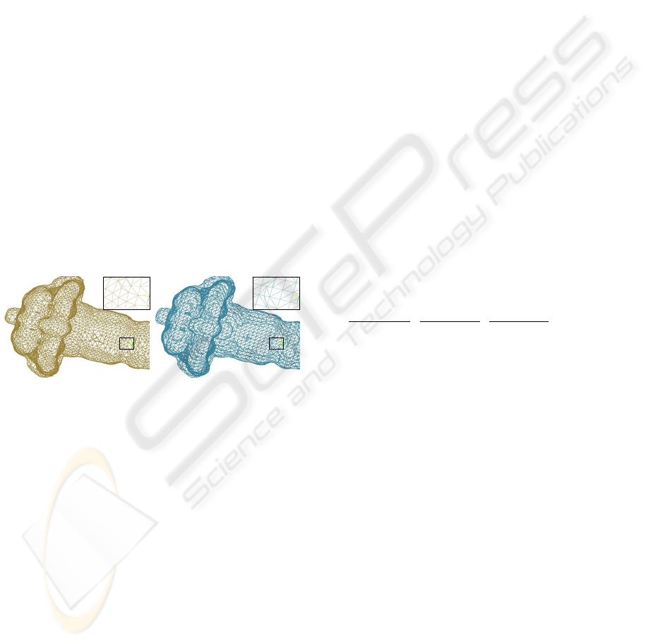
Figure 1: Better triangles in isosurface obtained using dual
contouring (left) than MC method (right) for the fuel dataset
(from http://www.volvis.org). The dual contouring result
is obtained from the isosurface points computed using our
method.
We present a dual isosurfacing method based on ray
intersection to determine isosurface points (Co et al.,
2003) (Parker et al., 1998). Since we are using a dual
approach, our algorithm has the typical advantages of
being able to extract sharp features, generating nice
triagulations, and being extendable to isosurface gen-
eration from adaptively refined grids without gener-
ating discontinuities. Moreover, our algorithm gen-
erates topologically correct isosurfaces including tun-
nel cases and multiple isosurface components per cell,
computes exact points on the isosurface with respect
to trilinear interpolation, and does not require any nor-
mal information such as Hermite data.
For the computation of the ray-isosurface intersec-
tion, we determine the minimum number of rays nec-
essary for finding sufficient number of points in each
cell to accomodate cases of single components, “mul-
tiple components” (i.e., disjoint pieces) of the isosur-
face as well as complex features like tunnels. We gen-
erate a look-up table based on all 31 topological con-
figurations of the cells (Lopes and Brodlie, 2003). In
Section 2, we provide a brief overview of trilinear
interpolation followed by the description of the ray-
intersection method. We formulate certain observed
properties of the cell diagonals used as rays in Sec-
tion 3, and enlist the rules used to optimize the ray-
intersections in Section 4.
For polygonization, we cluster isosurface points in
the neighborhood of each cell using connectivity in-
formation. Our simple strategy for connecting the
points also guarantees that multiple isosurface com-
ponents within each cell are rendered distinctly. We
explain the algorithm for computing isosurface points
and our simple polygonization strategy in Section 5.
2 BASIC MATHEMATICAL
FORMULATION
Let F (x, y, z) be the trivariate scalar field de-
fined over a structured rectilinear hexahedral
grid, and f(u, v, w) be its parametric rep-
resentation over the domain [x
min
,x
max
] ×
[y
min
,y
max
] × [z
min
,z
max
], i.e., F (x, y, z)=
f
x−x
min
x
max
−x
min
,
y −y
min
y
max
−y
min
,
z−z
min
z
max
−z
min
.
With (u
i
,v
j
,w
k
) being the parametric representa-
tion of the vertices of the cell (or voxel), for i, j, k, ∈
{0, 1}, the trilinear model f (u, v, w) is defined as
1
i=0
1
j=0
1
k=0
(1 − U
i
)(1 − V
j
)(1 − W
k
)f(u
i
,v
j
,w
k
) .
(1)
where U
i
= |u − u
i
|, V
j
= |v − v
j
|, and W
k
=
|w − w
k
|.
A hexahedral cell is represented by vertices with
minimum coordinates (u
0
,v
0
,w
0
)=(0, 0, 0) and
maximum coordinates (u
1
,v
1
,w
1
)=(1, 1, 1), re-
spectively. A point interior to the cell has parame-
ters (u, v, w) ∈ [0, 1]
3
. An isosurface associated with
value I, in parametric form and set form can be written
as
T (I)={(u, v, w):f (u, v, w)=I,0 ≤ u, v, w ≤ 1}
(2)
For our ray-intersection approach, the diagonals are
used as rays and points of intersection with the trilin-
ear isosurface are computed. The equation of a ray
r(t) from vertex V to vertex W is given by
r(t)= V + t(W − V), 0 ≤ t ≤ 1, (3)
USING RAY INTERSECTION FOR DUAL ISOSURFACING
35

where r(t), V and W can be represented as position
vectors or in the parametric form.
The point p being the intersection of a ray
and an implicitly defined isosurface satisfies Equa-
tions (1), (2) and (3). These conditions reduce to a
cubic equation in variable t, which corresponds to
the parametric representation of p on the ray, i.e.,
p = r(t), 0 ≤ t ≤ 1. The cubic equation can be
written as
G
3
t
3
+ G
2
t
2
+ G
1
t + G
0
=0. (4)
The computation of its coefficients G
0
,G
1
,G
2
and
G
3
is explained in Appendix A.
We solve Equation (4) using the analytical Car-
dan’s method (Nickalls, 1993) in case the equation
has points of inflexion or the numerical Newton-
Raphson method (Press et al., 1986) otherwise. The
intersection point(s) p is then computed using the real
root(s) of Equation (4) in Equation (3).
The roots of Equation (4) depend on the behavior of
the discriminant of the cubic or the reduced quadratic
equation, summarized in Table 1. Discriminant D
3
for Equation (4) is evaluated based on the point of in-
flexion (x
N
,y
N
) (Nickalls, 1993). We need to com-
pute
δ
2
=(G
2
2
− 3G
3
G
1
)/(9G
2
3
) ,
(x
N
,y
N
)=(−G
2
/(3G
3
),
G
3
x
3
N
+ G
2
x
2
N
+ G
1
x
N
+ G
0
), and
D
3
= y
2
N
− 4G
2
3
δ
3
. (5)
If G
3
=0, then the cubic equation reduces to a
quadratic one, and the quadratic discriminant D
2
de-
termines the nature of the roots.
D
2
= G
2
1
− 4G
2
G
0
. (6)
Table 1: Roots of governing cubic equation of trilinear func-
tion depending on its degree.
Degree Discriminant Nature of Roots
Cubic D
3
> 0 1 real,
2 imaginary
(G
3
=0) y
N
= D
3
=0 3 equal real
y
N
= D
3
=0 1 distinct real,
2 equal real
D
3
< 0 3 distinct real
Quadratic D
2
> 0 2 distinct real
(G
3
=0, D
2
=0 2 equal real
G
2
=0) D
2
< 0 2 imaginary
An intersecting ray can produce at most three iso-
points, by virtue of the governing cubic equation.
However, for most of the cases, either one or two so-
lutions result.
3 TERMINOLOGY
The sign of a vertex of a cell is positive, when the
scalar value at the vertex is greater than or equal to
a given isovalue, and negative otherwise. In the fol-
lowing, vertices will be denoted as “(+) vertices” and
“(-) vertices”, respectively.
We use cell diagonals to define rays, and based on
the sign of the vertices on the ray, we can have ei-
ther same-sign ended rays (+/+ or -/-) or different-
sign ended rays (+/- or -/+). In the former case there
are either zero or two solutions to the cubic equa-
tion for ray-isosurface intersection, and in the latter
there are either one or three solutions. Intuitively, an
odd number of intersections (or zeros) causes a sign
change, and an even number maintains the same sign
at the endpoints. We denote edges with same-sign
endpoints as “(+/+) or (-/-) edges”, and different-sign
ended edges as “(+/-) edges”, see Figure 2(a).
When a cell has more (+) vertices than (-) vertices,
the cell is said to be a positive cell (“(+) cell”). Simi-
larly, if the cell has more (-) vertices than (+) vertices,
it has a negative sign and is called a negative cell (“(-
) cell”). If both (+) vertices and (-) vertices are equal
in number then, the cell is a neutral cell (“(0) cell”),
with no sign. Examples of positive, negative and neu-
tral cells are shown in Figure 2(b).
A cell face with four same-sign ended diagonals
and four (+/-) edges is called an ambiguous face.An
ambiguous face separated with respect to a specific
sign (Chernyaev, 1995) (Nielson and Hamann, 1991)
means a contour on the face is a rectangular hyperbola
and the sign is that of the vertices in the quadrants
containing the hyperbola, see Figure 2(c). The sign,
with respect to which an ambiguous face is separated,
is determined using the asymptotic decider (Nielson
and Hamann, 1991). A face separated with respect to
positive sign will be denoted as “(+) ambiguous-face,”
and that with respect to negative sign will be denoted
as “(-) ambiguous-face.” Equations for the asymptotic
decider are given in Appendix A.
4 OPTIMIZATION
We use the trilinear function exhaustively for all pos-
sible configurations, and determine the topology of
the analytical isosurface. We can observe from the
analytical isosurface that there are cases where more
than one diagonal of the cell intersect the same iso-
surface component. Since evaluating the intersection
point requires a significant number of computational
operations, we optimize our algorithm by finding just
one point per disjoint piece of the isosurface within
the cell. We analyze each of the 31 cases from the ex-
haustive MC case-table (Chernyaev, 1995) (Nielson,
2003) (Lopes and Brodlie, 2003) to find the diagonals
used for intersection. A priori knowledge of diago-
nals for intersection helps us in easy computation of
isosurface points. The choice of diagonals for inter-
GRAPP 2006 - COMPUTER GRAPHICS THEORY AND APPLICATIONS
36
(+/+) Ray/Edge
(+/−) Ray/Edge
(−/−) Ray/Edge
V1(T10)V0(T00)
V
3(T01) V2(T11)
V7(T011)
V0(T000) V1(T100)
V6(T111
)
V2(T110)
V3(T010)
V4(T001) V5(T101)
(b)
(c)
(a)
(−) Cell
(+) Cell
(0) Cell
(d)
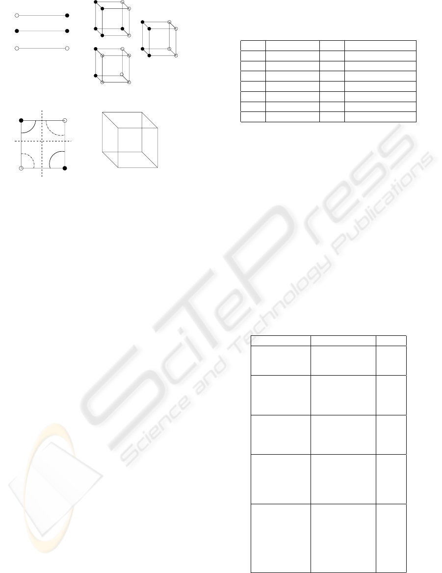
Figure 2: (a) Sign of ray/edge (b) Sign of cell (c) Ambigu-
ous face with the notations used for vertices and their scalar
values in bilinear interpolation. Solid contours occur when
the face is separated with respect to positive sign, and dot-
ted contours occur when with respect to negative sign (d)
Notation for cell vertices for trilinear interpolation. Black
and white vertices are positive and negative, respectively.
section depends on the number of ambiguous faces
of the cell, the sign of the ambiguous faces (Nielson
and Hamann, 1991), and the sign of the diagonals’
vertices. However, the condition of “one-point-per-
disjoint-component” is relaxed in the case of com-
plex features inside the cell, like tunnels, as sufficient
points are needed to capture the complexity of the
manifold.
We categorize the original 14 sign-configurations
(numbered 0 to 13) of the MC-case table to five cat-
egories, based on the number of ambiguous faces.
There can be only cases with zero, one, two, three,
and six ambiguous faces, by virtue of the possible
combinations of eight connected, signed vertices. We
observe that cells with same number of ambiguous
faces show similar choices for optimal number of
rays. We define rules to distinguish between differ-
ent topological configurations, and decide which di-
agonals are to be used for intersection. The configu-
ration are represented using numerical indices, which
were used in earlier works (Chernyaev, 1995) (Lopes
and Brodlie, 2003), of the form “x,” “x.y” or “x.y.z,”
where “x” is the sign configuration, “y” the topolog-
ical configuration, and subconfiguration “z.” Niel-
son (Nielson, 2003) showed analytically that there
can be just three “levels of characterization” for the
cell configurations. We use DeVella’s necklace test
(which leads to a positive result exclusively in the
presence of tunnels) (Nielson, 2003) in a few cases
to distinguish its different topological configurations.
DeVella’s necklace test checks if two vertices on a di-
agonal are internally connected (Nielson, 2003). Its
associated equations are explained in Appendix A.
Table 2: Types of diagonals for the 14 sign configurations
(for (+) cell, in case of non-(0) cells).
Case Diagonal types Case Diagonal types
0 4 (-/-) 7 3 (+/-), 1 (+/+)
1 1 (+/-), 3 (+/+) 8 4 (+/-)
2 2 (+/-), 2 (+/+) 9 4 (+/-)
3 2 (+/-), 2 (+/+) 10 2 (+/+), 2 (-/-)
4 1 (-/-), 3 (+/+) 11 4 (+/-)
5 3 (+/-), 1 (+/+) 12 2 (+/-), 1 (+/+), 1 (-/-)
6 1 (+/-), 2 (+/+), 13 4 (+/-), 1 (-/-)
The following subsections explain the choice of
the diagonals for each sign-configuration and their re-
spective topological configurations. Table 2 lists the
different types of diagonals in each of the sign con-
figurations, and Table 3 summarizes the rules for the
diagonals to be used for the five categories. In this
section, for cases of analysis of signed cells, we will
use the example of a (+) cell, and similar analysis can
be extended to a (-) cell, by interchanging the signs of
the diagonals, ambiguous faces and the cell.
Table 3: Rules used to choose diagonals in 31 topological
configurations based on the number of ambiguous faces (for
(+) cell, in case of non-(0) cells). Notations: “AF” implies
ambiguous faces, “IP” means isosurface points, T stands for
tunnel points, DS represents disjoint surface, and (+/-)
C
(in
case 13) is the (+/-) diagonal through the common vertices
of 3 (+) ambiguous faces and 3 (-) ambiguous faces, respec-
tively.
Cases Diagonals/Rays #IP.
0 AF: 1, 2, 5, For x (=4),1 (+/-) 1
8, 9, 11, For 4.1, 1 (-/-) 2
4 (4.1, 4.2) For 4.2, 2 (+/+) 4(T)
1 AF: 3 (3.1,3.2), For 3.1, 2 (+/-) 2
6 (6.1.1, 6.1.2, For 6.1.1, 1 (-/-) 2
6.2) For 6.1.2, 2 (+/+) 4 (T)
For x.2, 1 (+/-) 1
2 AF: 10,12 For x.1.1, 1 (+/+) 1
(x.1.1, x.1.2, x.2) For x.1.2, 2 (-/-) 4(T)
(case of 2 (+) AF. For 10.2, 1(+/+) 1
for x.1.z) For 12.2, 1 (+/-) 1
3 AF: 7 (7.1, 7.2, For 7.1, 3 (+/-) 3
7.3, 7.4.1, 7.4.2) For 7.2, 2 (+/-) 2
For 7.3, 1 (+/-) 1
For 7.4.1, 1 (+/+) 2
For 7.4.2, 3 (+/-) 3(T)
6 AF: 13 (13.1, For 13.1, 4 (+/-) 4
13.2, 13.3, 13.4, For 13.2, 3 (+/-) 3
13.5.1,13.5.2) For 13.3, 2 (+/-) 2
For 13.4, 1 (+/-) 1
For 13.5.1, 1(+/-)
C
3
For 13.5.2, 1(+/-)
C
1(DS)
& 3(+/-) &3(T)
Cases without Ambiguous Faces. Sign configura-
tions 0, 1, 2, 4, 5, 8, 9, and 11 have no ambiguous
faces, see Figure 3. We ignore case 0 in our diagonal
USING RAY INTERSECTION FOR DUAL ISOSURFACING
37
analysis, as it does not intersect the isosurface. Except
for case 4, these cases have just one topological con-
figuration and one isosurface component each. It can
be seen from the analytical trilinear surface, shown in
Figure 3, that cases 1, 2, 5, 8, 9, and 11 can use a
(+/-) diagonal for intersection.
In case 4, two different topologies occur, depend-
ing on whether the vertices on the (-/-) diagonal are
“internally connected”. In configuration 4.1, the con-
tour forms disjoint surfaces, and in configuration 4.2,
they are internally connected to form a tunnel. We use
DeVella’s necklace test to distinguish between the two
subconfigurations (Nielson, 2003). For configuration
4.1, the (-/-) diagonal is used for intersection, and for
configuration 4.2, 2 of the 3 (+/+) diagonals are used
to obtain multiple points for defining the tunnel.
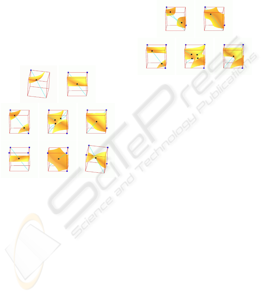
case 1
case 2
case 4.1
case 4.2
case 5
case 8
case 9
case 11
Figure 3: Topological configurations with no ambiguous
faces: trilinear model in yellow-orange, isopoints in black,
positive nodes in blue, rays in cyan.
Cases with One Ambiguous Face. Sign configu-
rations 3 and 6 have one ambiguous face each, as
shown in Figure 4. If a (+) cell has a (+) ambigu-
ous face (i.e., the same sign as the cell), then a sin-
gle isosurface component occurs; and if the (+) cell
has a (-) ambiguous face, then two isosurface com-
ponents occur. 3.1 and 6.1 are configurations where
there are two disjoint isosurface pieces, and 3.2 and
6.2 are configurations with a single isosurface piece.
In the case of 6.1, a same-sign ended diagonal inter-
sects the isosurfaces, and the vertices on the diagonal
may be internally connected (Nielson, 2003) to form
a tunnel. Thus, there are two subconfigurations 6.1.1
and 6.1.2, based on the absence and presence of a tun-
nel, respectively, and they are distinguished using the
DeVella’s necklace test. In the case of two isosurface
components and no tunnels (cases 3.1 and 6.1.1), for
a (+) cell, a (-/-) diagonal is used to obtain two inter-
section points. In case of 3.1, where there are no (-/-
) diagonals, two (+/-) diagonals are used to obtain an
intersection point each. For case 6.1.2, both (+/+) di-
agonals are used to obtain four intersection points on
the tunnel. In the case of a single isosurface compo-
nent, in cases 3.2 and 6.2, a (+/-) diagonal is used to
determine an intersection point.
case 3.1
case 3.2
case 6.1.1
case 6.1.2
case 6.2
Figure 4: Topological configurations with one ambiguous
face: trilinear model in yellow-orange, isopoints in black,
positive nodes in blue, rays in cyan.
Cases with Two Ambiguous Faces. Sign configu-
rations 10 and 12 have two ambiguous faces, see Fig-
ure 5. In this case, there are two topological config-
urations based on the signs of the ambiguous faces.
If both ambiguous faces are separated with respect to
the same sign, then a same-sign ended diagonal of the
cell can intersect two disjoint isosurface pieces (cases
10.1.1 and 12.1.1), or the vertices of the diagonal can
be internally connected to form tunnels (cases 10.1.2
and 12.1.2). If the ambiguous faces are separated
with respect to different signs, then a single isosur-
face piece occurs (cases 10.2 and 12.2). In the case of
a single isosurface component (cases 10.2 and 12.2),
a (+/-) diagonal is used to obtain a single intersection
point. In the case of disjoint surfaces in a configura-
tion with two (+) ambiguous faces, a (+/+) diagonal
is used to obtain two intersection points. Similarly, in
the case of two (-) ambiguous faces and disjoint sur-
faces, a (-/-) diagonal is used. In the case of a tunnel
and two (+) ambiguous faces, two (-/-) diagonals (in
case 10.1.2) or one (-/-) diagonal and two (+/-) diag-
onals (in case 12.1.2) are used. A similar extension is
done for a tunnel and two (-) ambiguous faces.
Cases with Three Ambiguous Faces. Sign config-
uration 7 has three ambiguous faces, see Figure 6. In
a (+) cell, there are four possibilities of sign combina-
tions of the three ambiguous faces, represented in set
form as (1) (+,+,+), (2) (+,+,-), (3) (+,-,-), and (4) (-,-,-
). In configuration 7.1, there are three (+) ambiguous
faces, which leads to three disjoint surfaces, and three
(+/-) diagonals are used as rays. In configuration 7.2
with two (+) ambiguous faces and one (-) ambiguous
face, two disjoint surfaces are formed. In this case,
two (+/-) diagonals are used through the (+) vertices
GRAPP 2006 - COMPUTER GRAPHICS THEORY AND APPLICATIONS
38
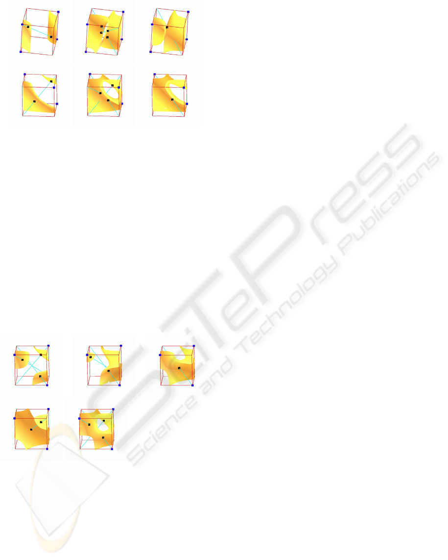
case 10.1.1
case 10.1.2
case 10.2
case 12.1.1
case 12.1.2
case 12.2
Figure 5: Topological configurations with two ambiguous
faces: trilinear model in yellow-orange, isopoints in black,
positive nodes in blue, rays in cyan.
in one of the (+) ambiguous faces. These rays are
specifically used to ensure that one obtains one inter-
section point per surface. In configuration 7.3, with
one (+) ambiguous face and two (-) ambiguous faces,
one surface occurs, and any one of the (+/-) diagonals
can be used. In configuration 7.4 with three (-) am-
biguous faces, there are two disjoint surfaces. How-
ever, in this case the vertices on the (+/+) diagonal
can be internally connected to form a tunnel. Thus,
there are two topological subconfigurations, 7.4.1 and
7.4.2, with two disjoint surfaces and with a tunnel, re-
spectively. In case 7.4.1, a (+/+) diagonal is used to
obtain two intersection points. In case 7.4.2, all three
(+/-) diagonals are used to obtain three points on the
tunnel.
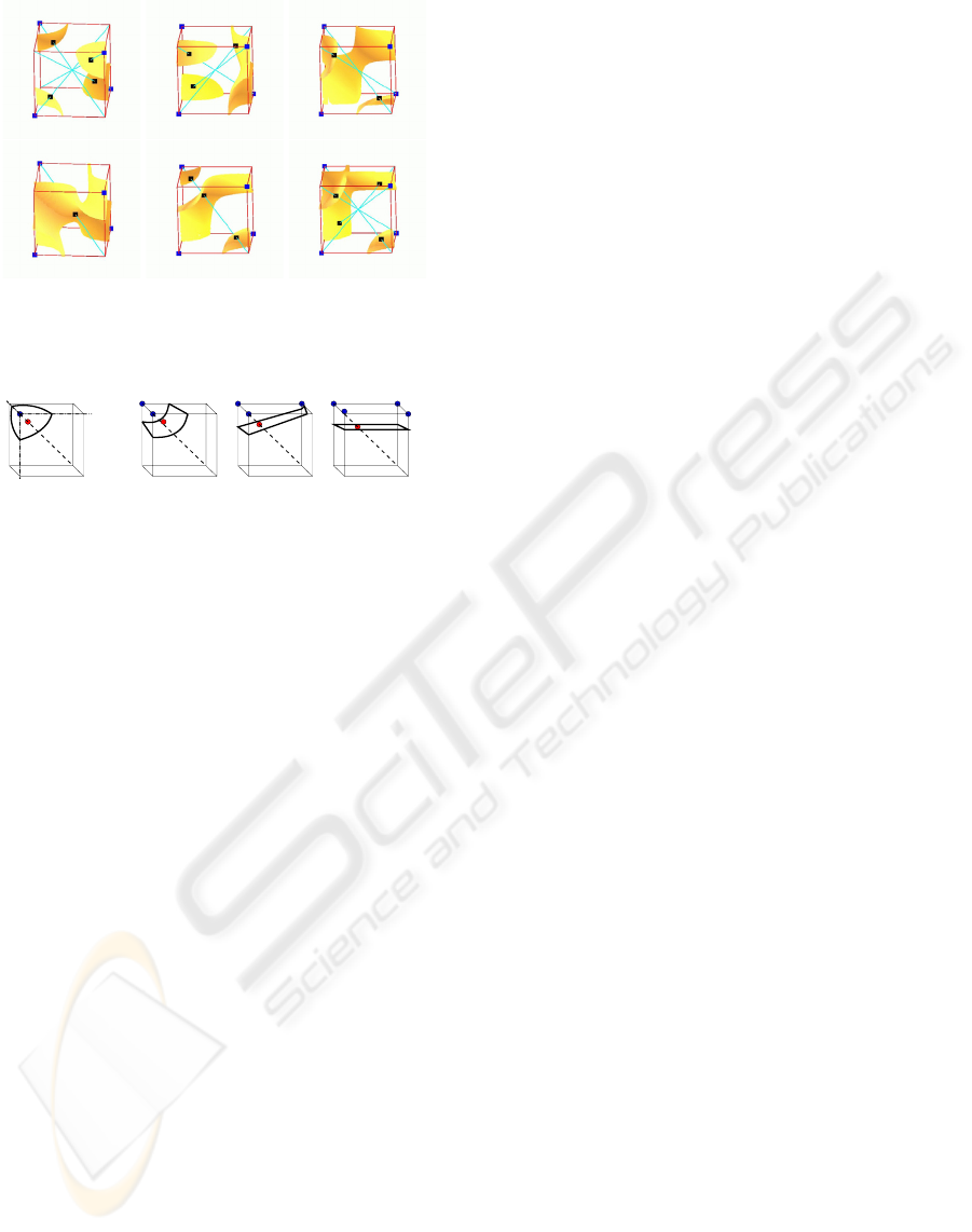
case 7.1
case 7.2
case 7.3
case 7.4.1
case 7.4.2
Figure 6: Topological configurations with three ambiguous
faces: trilinear model in yellow-orange, isopoints in black,
positive nodes in blue, rays in cyan.
Cases with Six Ambiguous Faces. Sign configura-
tion 13 has six ambiguous faces and four (+/-) diag-
onals, see Figure 7. There are seven possibilities of
sign combinations of the six ambiguous faces, which
are, (1) (+,+,+,+,+,+), (2) (+,+,+,+,+,-), (3) (+,+,+,+,-
,-), (4) (+,+,+,-,-,-), (5) (+,+,-,-,-,-), (6) (+,-,-,-,-,-),
and (7) (-,-,-,-,-,-). However, this can be reduced to
four cases, as (1) and (7), (2) and (6), and (3) and (5)
are pairs of mirror cases.
In configuration 13.1 with all six (+) ambiguous
faces, four disjoint surfaces are formed and all the
diagonals are used. In configuration 13.2 with five
(+) ambiguous faces and one (-) ambiguous face,
three disjoint surfaces are formed. Except for a diag-
onal through one of the two (+) vertices in the (-) am-
biguous face, all the other three (+/-) diagonals are
used. Specific rays are used in order to generate one
intersection point per surface piece. In configuration
13.3 with four (+) ambiguous faces and two (-) am-
biguous faces, there are two disjoint surfaces. We find
the (+) vertex that is common to all three (+) ambigu-
ous faces, and the (+/-) diagonal through this vertex is
one of the two rays used for isosurface computations.
Any one of the remaining three diagonals is used as
the second ray. In case of equal number of (+) and (-
) ambiguous faces, suppose A and B are two vertices
of the cell, such that A is common to all (+) ambigu-
ous faces and B is common to all (-) ambiguous faces.
AB is a diagonal of the cell. There are two possibil-
ities of this configuration depending on the signs of
A and B. In configuration 13.4, the sign of the com-
mon vertex is different from that of the faces (i.e., A
is a (-) vertex and B, a (+) vertex), and in configura-
tion 13.5, it is the same as that of the faces (i.e., A is a
(+) vertex and B is a (-) vertex). In configuration 13.4,
there is one isosurface piece, and any one of the four
(+/-) diagonals can be used. In configuration 13.5,
there can be three disjoint surfaces, which can reduce
to two, in case of internal connection. In configuration
13.5.1, there are three disjoint surfaces, and three in-
tersection points are obtained from the (+/-) diagonal
through the common vertex of the three same-signed
ambiguous faces (i.e., AB). This is the unique case
where a (+/-) ray leads to three solutions. In config-
uration 13.5.2, two disjoint surfaces occur, of which
one is a tunnel. Hence, the diagonal through the com-
mon vertex of the three same-signed ambiguous faces
(AB) is used as a ray. The remaining three diagonals
are used as rays to find isosurface points for the tun-
nel. Thus, all four diagonals are used in case 13.5.2.
However the difference in the diagonals used for the
two surfaces is to be stored for connectivity during
polygonization.
5 ALGORITHM
Our algorithm involves two major steps: (1) isosur-
face point computation and (2) triangulating the iso-
surface points.
We generate a look-up table for the choice of diag-
onals in each topological configuration. This a priori
information saves a lot of computation time. Our al-
gorithm generates a vector or list of all the heteroge-
neous cells, and evaluates the topological configura-
tion of each cell. Based on its configuration, the di-
USING RAY INTERSECTION FOR DUAL ISOSURFACING
39
case 13.1
case 13.2
case 13.3
case 13.4
case 13.5.1
case 13.5.2
Figure 7: Topological configurations with six ambiguous
faces: trilinear model in yellow-orange, isopoints in black,
positive nodes in blue, rays in cyan.
e
A
e
e
(a)
A
B
(b)
B
A
B B
A
B
B
Figure 8: (a) Associations of isosurface point (in red) with
vertex A (in blue), which is the endpoint of the intersect-
ing diagonal closer to the isosurface (curved lines), and
the edges “e” containing A; (b) Configurations where iso-
surface point is associated with vertex A on the intersect-
ing diagonal, and additional associations between isosur-
face point and vertices, B, are made. Blue cell vertices are
associated with the red isosurface point, the bold dotted line
is the intersecting diagonal, and the curved boundary is the
isosurface.
agonals specified in the look-up table are used to find
out the isosurface points.
We associate each isosurface point with an edge of
the cell, when the edge contains the end-point of the
diagonal (used for the respective intersection) near-
est to the isosurface point, as shown in Figure 8(a).
Certain configurations require additional associations
with vertices to make appropriate connectivity, see
Figure 8(b). The isosurface point is then associ-
ated with all the edges containing its associated ver-
tices. An edge is shared by four neighboring cells,
and thus, it can get associated with three or four
isosurface points (which are in different cells that
share the edge). The isosurface points associated
with an edge are connected to form one or two dis-
tinct non-overlapping triangles. This strategy is sim-
ilar to the connectivity used in earlier dual isosurfac-
ing works (Gibson, 1998) (Ju et al., 2002), and it re-
sults in a triangular mesh. In cases of tunnels, we
treat them as isolated cells with no neighbors and em-
ploy polygonization for its isosurface points indepen-
dently (Lopes and Brodlie, 2003).
We have applied the algorithm on some standard
datasets. Figure 1 and 9 show the resulting isosurfaces
in comparison to isosurfaces extracted using a state-
of-the-art MC method. Superposition of both surfaces
show their similarity.
6 CONCLUSIONS
We have presented a dual isosurfacing method based
on ray intersection to determine isosurface points.
Apart from having the typical advantages of dual ap-
proaches (being able to extract sharp features, gener-
ating nice triagulations, and being extendable to iso-
surface generation from adaptively refined grids with-
out generating discontinuities), our algorithm gener-
ates topologically correct isosurfaces including tun-
nel cases and multiple isosurface components per cell,
computes exact points on the isosurface with respect
to trilinear interpolation, and does not require any nor-
mal information such as Hermite data.
The computation times of the points on the iso-
surface is considerably fast and comparable to the
performance of an MC algorithm. For the examples
shown in Figure 9, the computation times were 0.96s,
1.67s, 2.36s, and 4.08s (top to bottom). The perfor-
mance depends on the number of tunnel cases (e. g. 42
and 67 for the latter two examples). However, The
polygonization step still needs to be optimized. Using
efficient data structures like kd-trees (Greß and Klein,
2003) would improve the performance of this method
tremendously. We also plan to generalize our method
for adaptive grids or irregular meshes. Other future
directions also include developing a meshless surface
construction from the isosurface points. Moreover,
we plan to analytically calculate the translation in
the axis, using the analytical trilinear model (Nielson,
2003), and employ the designated diagonals for inter-
section.
ACKNOWLEDGMENTS
This work was supported by the National Science
Foundation under contract ACI9624034 (CAREER
Award), through the Large Scientific and Software
Data Set Visualization (LSSDSV) program under
contract ACI9982251, through the National Part-
nership for Advanced Computational Infrastructure
(NPACI) and a large Information Technology Re-
search (ITR) grant; the National Institutes of Health
under contract P20 MH60975-06A2, funded by the
National Institute of Mental Health and the National
Science Foundation; and the U.S. Bureau of Reclama-
tion. We thank the members of the Institute for Data
Analysis and Visualization (IDAV) at the University
of California, Davis.
GRAPP 2006 - COMPUTER GRAPHICS THEORY AND APPLICATIONS
40
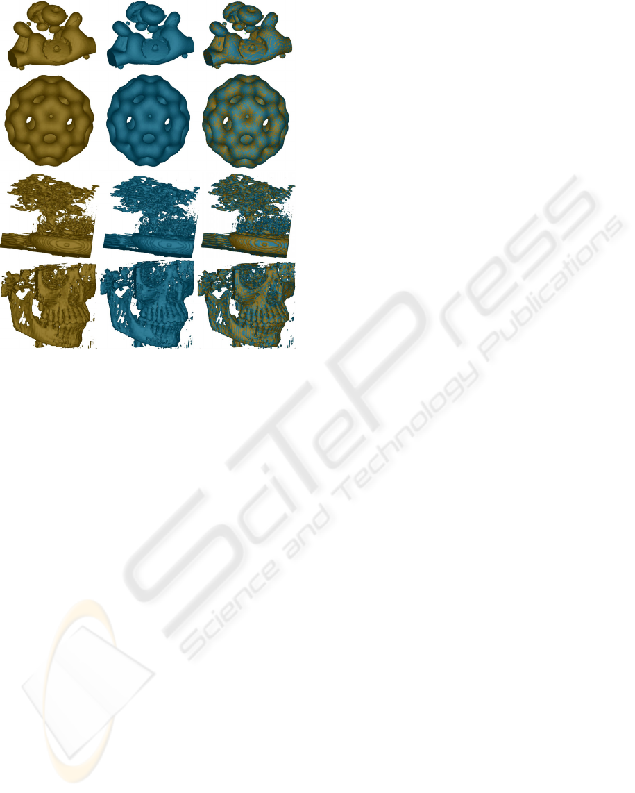
Figure 9: Dual contouring result (left), MC result (middle),
and comparisons of both surfaces by superposition for reg-
ular datasets of size 64x64x64 of Neghip (top) and Buck-
yball (second), and of size 256x256x256 (rendered in 1:4)
of Bonsai (third) and Skull (bottom). (Datasets available at
http://www.volvis.org.)
REFERENCES
Chernyaev, E. V. (1995). Marching cubes 33: Con-
struction of topologically correct isosurfaces.
In Technical Report CERN CN 95-17. CERN.
http://citeseer.ist.psu.edu/4145.html.
Co, C. S., Hamann, B., and Joy, K. I. (2003). Iso-splatting:
A point-based alternative to isosurface visualization.
In Rokne, J., Wang, W., and Klein, R., editors, Pro-
ceedings of the Eleventh Pacific Conference on Com-
puter Graphics and Applications - Pacific Graphics
2003, pages 325–334.
Gibson, S. F. F. (1998). Constrained elastic surface nets:
Generating smooth surfaces from binary segmented
data. In MICCAI ’98: Proceedings of the First In-
ternational Conference on Medical Image Computing
and Computer-Assisted Intervention, pages 888–898,
London, UK. Springer-Verlag.
Greß, A. and Klein, R. (2003). Efficient representation and
extraction of 2-manifold isosurfaces using kd-trees. In
Proceedings of The Eleventh Pacific Conference on
Computer Graphics and Applications - Pacific Graph-
ics 2003. IEEE CS Press.
Ju, T., Losasso, F., Schaefer, S., and Warren, J. (2002). Dual
contouring of hermite data. In Proceedings of the 29th
annual conference on Computer graphics and inter-
active techniques - SIGGRAPH 2002, pages 339–346.
ACM Press.
Kobbelt, L., Botsch, M., Schwanecke, U., and Seidel,
H.-P. (2001). Feature sensitive surface extraction
from volume data. In Proceedings of the 28th an-
nual conference on Computer graphics and interac-
tive techniques-SIGGRAPH 2001, pages 57–66. ACM
Press.
Lopes, A. and Brodlie, K. (2003). Improving the robust-
ness and accuracy of the marching cubes algorithm
for isosurfacing. IEEE Transactions on Visualization
and Computer Graphics, 9(1):16–29.
Lorensen, W. E. and Cline, H. E. (1987). Marching cubes:
A high resolution 3d surface construction algorithm.
In Proceedings of the 14th annual conference on
Computer graphics and interactive techniques - SIG-
GRAPH 1987, pages 163–169. ACM Press.
Nickalls, R. W. D. (1993). A new approach to solving the
cubic: Cardan’s solution revealed. The Mathematical
Gazette, 77:354–359.
Nielson, G. M. (2003). On marching cubes. IEEE
Transactions on Visualization and Computer Graph-
ics, 9(3):283–297.
Nielson, G. M. (2004). Dual marching cubes. In VIS ’04:
Proceedings of the conference on Visualization ’04,
pages 489–496, Washington, DC, USA. IEEE Com-
puter Society.
Nielson, G. M. and Hamann, B. (1991). The asymptotic
decider: resolving the ambiguity in marching cubes.
In Nielson, G. M. and Rosenblum, L. J., editors, Pro-
ceedings of IEEE Conference on Visualization 1991,
pages 83–91. IEEE Computer Society Press.
Parker, S., Shirley, P., Livnat, Y., Hansen, C., and Sloan,
P.-P. (1998). Interactive ray tracing for isosurface ren-
dering. In VIS ’98: Proceedings of the conference on
Visualization ’98, pages 233–238, Los Alamitos, CA,
USA. IEEE Computer Society Press.
Press, W. H., Flannery, B. P., Teukolsky, S. A., and Vet-
terling, W. T. (1986). Numerical Recipes: The Art
of Scientific Computing. Cambridge University Press,
first edition.
Schaefer, S. and Warren, J. D. (2004). Dual marching cubes:
Primal contouring of dual grids. In Pacific Conference
on Computer Graphics and Applications, pages 70–
76.
APPENDIX A
The parametric equation for the isosurface (Equation (2)) in
Section 2 can be rewritten as:
F
i
(u, v, w, I)=Auvw+Buv +Cvw+Dwv +Eu+Fv+Gw+H,
(7)
where I is the given isovalue and T
ijk
= f(u
i
,v
j
,w
k
)
denote the vertices of a cell, see Figure 2(d). The values of
coefficients are A = −T
000
+ T
010
− T
110
+ T
100
+ T
001
−
T
011
+ T
111
− T
101
, B = T
000
− T
010
− T
100
+ T
110
,
USING RAY INTERSECTION FOR DUAL ISOSURFACING
41

C = T
000
− T
010
− T
100
+ T
110
, D = T
000
− T
100
−
T
001
+ T
101
, E = −T
000
+ T
100
, F = −T
000
+ T
010
, G =
−T
000
+ T
001
, and H = T
000
− I. Let (u
r
0
,v
r
0
,w
r
0
) and
(u
r
1
,v
r
1
,w
r
1
) be the endpoints of the ray (in parametric
form). The intersection point is given, in parametric form,
by (u
∗
,v
∗
,w
∗
)=(u
r
0
+t∆u
r
,v
r
0
+t∆v
r
,w
r
0
+t∆w
r
),
where ∆u
r
= u
r
1
− u
r
0
, ∆v
r
= v
r
1
− v
r
0
, ∆w
r
=
w
r
1
− w
r
0
, and parameter t, 0 ≤ t ≤ 1, computed using
the ray equation (Equations (3) and (4)). The coefficients
G
0
, G
1
, G
2
, and G
3
, of the cubic equation (Equation (4))
are obtained by using Equation (7), F
i
(u
∗
,v
∗
,w
∗
,I)=0.
G
0
= F
i
(u
r
0
,v
r
0
,w
r
0
,I),
G
1
= A(u
r
0
v
r
0
∆w
r
+ v
r
0
w
r
0
∆u
r
+ w
r
0
u
r
0
∆v
r
)+
B(v
r
0
∆u
r
+ u
r
0
∆v
r
)+C(w
r
0
∆v
r
+ v
r
0
∆w
r
)+
D(u
r
0
∆w
r
+ w
r
0
∆u
r
)+E∆u
r
+ F ∆v
r
+ G∆w
r
,
G
2
= A(u
r
0
∆v
r
∆w
r
+ v
r
0
∆w
r
∆u
r
+ w
r
0
∆u
r
∆v
r
)+
B∆u
r
∆v
r
+ C∆v
r
∆w
r
+ D∆w
r
∆u
r
, and
G
3
= A∆u
r
∆v
r
∆w
r
.
For the asymptotic decider test (Nielson and Hamann,
1991), one uses bilinear interpolation to compute a value
V = T
00
T
11
− T
01
T
10
− I(T
00
+ T
11
− T
01
− T
10
), for a
given isovalue I, see Figure 2(c). The test states that when
V<0, the isocontour is a rectangular hyperbola in the first
and third quadrants, and when V>0, then the isocontour is
a rectangular hyperbola in the second and fourth quadrants.
DeVella’s necklace test states that if G[F
i
] < 0 and
DisC[F
i
] > 0, then there exists a tunnel in the cell (Niel-
son, 2003) for values G[F
i
] and Disc[F
i
] obtained from the
coefficients of the isosurface equation(Equation (7)):
G[F
i
]=(AE − BD)(AF − BC )(AG − CD),
DisC [F
i
]=(AH)
2
+(BG)
2
+(CE)
2
+(DF )
2
−2ABGH − 2ACEH − 2ADF H − 2BCEG
−2BDF G − 2CDEF +4AE F G +4BCDH .
GRAPP 2006 - COMPUTER GRAPHICS THEORY AND APPLICATIONS
42
