
A PROGRESSIVE REFINEMENT APPROACH
FOR THE VISUALISATION OF IMPLICIT SURFACES
Manuel N. Gamito
∗
Department of Computer Science
The University of Sheffield
Steve C. Maddock
Department of Computer Science
The University of Sheffield
Keywords:
Affine arithmetic, implicit surface, progressive refinement, ray casting.
Abstract:
Visualising implicit surfaces with the ray casting method is a slow procedure. The design cycle of a new
implicit surface is, therefore, fraught with long latency times as a user must wait for the surface to be rendered
before being able to decide what changes should be introduced in the next iteration. In this paper, we present
an attempt at reducing the design cycle of an implicit surface modeler by introducing a progressive refinement
rendering approach to the visualisation of implicit surfaces. This progressive refinement renderer provides a
quick previewing facility. It first displays a low quality estimate of what the final rendering is going to be
and, as the computation progresses, increases the quality of this estimate at a steady rate. The progressive
refinement algorithm is based on the adaptive subdivision of the viewing frustrum into smaller cells. An
estimate for the variation of the implicit function inside each cell is obtained with an affine arithmetic range
estimation technique. Overall, we show that our progressive refinement approach not only provides the user
with visual feedback as the rendering advances but is also capable of completing the image faster than a
conventional implicit surface rendering algorithm based on ray casting.
1 INTRODUCTION
Implicit surfaces play an important role in Com-
puter Graphics. Surfaces exhibiting complex topolo-
gies, i.e. with many holes or disconnected pieces,
can be easily modelled in implicit form (Desbrun and
Gascuel, 1995; Whitaker, 1998; Foster and Fedkiw,
2001). An implicit surface is defined as the set of all
points x that verify the condition f(x)=0for some
function f(x) from R
3
to R. Modelling with implicit
surfaces amounts to the construction of an appropriate
function f (x) that will generate the desired surface.
Rendering algorithms for implicit surfaces can be
broadly divided into meshing algorithms and ray cast-
ing algorithms. Meshing algorithms convert an im-
plicit surface to a polygonal mesh format, which
can be subsequently rendered in real time with mod-
ern graphics processor boards (Lorensen and Cline,
1987; Bloomenthal, 1988; Velho, 1996). Ray cast-
ing algorithms bypass mesh generation entirely and
compute instead the projection of an implicit surface
on the screen by casting rays from each pixel into
∗
Supported by grant SFRH/BD/16249/2004 from
Fundac¸
˜
ao para a Ci
ˆ
encia e a Tecnologia, Portugal.
three-dimensional space and finding their intersection
with the surface (Roth, 1982; Hin et al., 1989).
Our ultimate goal is to use implicit surfaces as a
tool to model and visualise realistic procedural plan-
ets over a very wide range of scales. The function
f(x) that generates the surface terrain for such a
planet must have fractal scaling properties and exhibit
a large amount of small scale detail. Examples of this
type of terrain generating function can be found in
the Computer Graphics literature (Ebert et al., 2003).
In our planet modelling scenario, meshing algorithms
are too cumbersome as they generate meshes with a
very high polygon count in order to preserve all the
visible surface detail. Furthermore, as the viewing
distance changes, the amount of surface detail varies
accordingly and the whole polygon mesh needs to be
regenerated. For these reasons, we have preferred a
ray casting approach because of its ability to render
the surface directly without the need for an interme-
diate polygonal representation.
The visualisation of an implicit surface with ray
casting is not without its problems, however. When
the surface is complex, many iterations have to be
performed along each ray in order to locate the inter-
section point with an acceptable accuracy (Mitchell,
26
N. Gamito M. and C. Maddock S. (2006).
A PROGRESSIVE REFINEMENT APPROACH FOR THE VISUALISATION OF IMPLICIT SURFACES.
In Proceedings of the First International Conference on Computer Graphics Theory and Applications, pages 26-33
DOI: 10.5220/0001350400260033
Copyright
c
SciTePress

1990). Imaging an implicit surface with ray casting
can then become a slow procedure. This is further
compounded by the fact that an anti-aliased image re-
quires that many rays be shot for each pixel (Cook,
1989).
We propose to alleviate the long rendering times
associated with the modelling and subsequent ray
casting of complex fractal surfaces by providing a
quick previewer based on a progressive refinement
rendering principle. The idea of progressive refine-
ment for image rendering was first formalised in
1986 (Bergman et al., 1986). Progressive refinement
rendering has received much attention in the fields of
radiosity and global illumination (Cohen et al., 1988;
Guo, 1998; Farrugia and Peroche, 2004). Progres-
sive refinement approaches to volume rendering have
also been developed (Laur and Hanrahan, 1991; Lip-
pert and Gross, 1995). Our previewer uses progres-
sive rendering to visualise an increasingly better ap-
proximation to the final implicit surface. It allows the
user to make quick editing decisions without having
to wait for a full ray casting solution to be computed.
Because the rendering is progressive, the previewer
can be terminated as soon as the user is satisfied or
not with the look of the surface. The previewer is also
capable of completing the image in a shorter amount
of time than it would take for a ray caster to render
the same image by shooting a single ray through the
centre of each pixel.
2 RENDERING WITH
PROGRESSIVE REFINEMENT
The main stage of our method consists in the binary
subdivision of the space, visible from the camera, into
progressively smaller cells that are known to strad-
dle the boundary of the surface. The subdivision
mechanism stops as soon as the projected size of a
cell on the screen becomes smaller than the size of
a pixel. Information about the behaviour of the im-
plicit function f(x) inside a cell is returned by evalu-
ating the function with affine arithmetic (Comba and
Stolfi, 1993). Affine arithmetic is a framework for
evaluating algebraic functions with arguments that are
bounded but otherwise unknown. It is a generalisation
of the older interval arithmetic framework (Moore,
1966). Affine arithmetic, when compared against in-
terval arithmetic, is capable of returning much tighter
estimates for the variation of a function, given input
arguments that vary over the same given range. Affine
arithmetic has been used with success in an increasing
number of Computer Graphics problems, including
the ray casting of implicit surfaces (Heidrich and Sei-
del, 1998; Heidrich et al., 1998; de Figueiredo, 1996;
Junior et al., 1999; de Figueiredo et al., 2003). We use
a recently developed form of affine arithmetic that is
termed reduced affine arithmetic (Gamito and Mad-
dock, 2005). Reduced affine arithmetic, in the context
of ray casting implicit surfaces made from procedural
fractal functions, returns the same results as standard
affine arithmetic while being faster to compute and
requiring smaller data structures.
The procedure for rendering implicit surfaces with
progressive refinement can be broken down into the
following steps:
1. Build an initial cell coincident with the camera’s
viewing frustrum. The near and far clipping planes
are determined so as to bound the implicit surface.
2. Recursively subdivide this cell into smaller cells.
Discard cells that do not intersect with the implicit
surface. Stop subdivision if the size of the cell’s
projection on the image plane falls below the size
of a pixel.
3. Assign the shading value of a cell to all pixels that
are contained inside its projection on the image
plane. The shading value for a cell is taken from
the evaluation of the shading model at the centre
point of the cell.
The Rayshade public domain ray tracer imple-
ments a previewing tool that traces rays at the corners
of rectangular regions in the image and subdivides
these regions based on their estimated contrast (Kolb,
1992). Since the ray casting of implicit surfaces is
one instance of the more general ray tracing problem,
the same previewing mechanism could be used here.
In a ray tracer, the process of ray-surface intersection
is performed independently for each ray, with no in-
formation being shared between neighbouring rays.
When a cell is subdivided, on the other hand, the in-
formation about the implicit surface contained in that
cell is refined and passed down to the child cells.
A previewer for implicit surfaces that uses cell sub-
division will, therefore, converge more quickly than
a generic previewer that uses subdivision in image
space, as implemented in Rayshade.
Another previewing method for implicit surfaces
with some similarities to ours was briefly described as
part of a larger work (de Figueiredo and Stolfi, 1996).
A subdivision of space using an octree is proposed to
track the boundary of the surface with increasing ac-
curacy. Surface visibility is determined by a painters
algorithm whereby the octree is traversed in back to
front order, relative to the camera, as the cells are ren-
dered on the screen. Our method is more efficient and
less memory intensive in that only the cells that are
known to be visible from the camera are considered.
No time is wasted tracking and subdividing cells that
lie on hidden portions of the surface. The following
sections will explain how each of the steps in our ren-
dering method work.
A PROGRESSIVE REFINEMENT APPROACH FOR THE VISUALISATION OF IMPLICIT SURFACES
27
2.1 Reduced Affine Arithmetic
A variable is represented with reduced affine arith-
metic (rAA) as a central value plus a series of noise
symbols. In contrast to the standard affine arithmetic
model, the number of noise symbols is constant, be-
ing given by the fundamental degrees of freedom of
the problem under consideration (Gamito and Mad-
dock, 2005). In the rendering method that is being
described in this paper, the degrees of freedom are the
three parameters necessary to locate any point inside
the viewing frustrum of the camera. These parameters
are the horizontal distance u along the image plane,
the vertical distance v along the same image plane
and the distance t along the ray that passes through
the point at (u, v). A rAA variable ˆa has, therefore,
the following representation:
ˆa = a
0
+ a
u
e
u
+ a
v
e
v
+ a
t
e
t
+ a
k
e
k
. (1)
The extra noise symbol e
k
is included to account
for uncertainties in the ˆa variable that are not shared
with any other variable. Non-linear operations on
rAA variables are performed by updating the a
u
, a
v
and a
t
noise coefficients with new uncertainties re-
lated to the u, v and t view frustrum distances and
clumping all other uncertainties into the a
k
coeffi-
cient.
For an implicit surface, the vector f(x) at some
point x in space can be described in rAA format as
a tuple of three cartesian coordinates, with the repre-
sentation in (1), and where the noise symbols e
u
, e
v
and e
t
are shared between the coordinates. Each co-
ordinate has its own independent noise symbol e
k
i
,
with i =1, 2, 3. The rAA representation
ˆ
x of the
vector x describes not a point but a region of space
spanned by the uncertainties associated with its three
coordinates. Evaluation of the expression ˆy = f(
ˆ
x)
leads to a range estimate ˆy for the variation of f(
ˆ
x) in-
side the region spanned by
ˆ
x. Knowing ˆy, the average
value ¯y and the variance y for that range estimate
can be computed as follows, based on the representa-
tion in (1) for an rAA variable:
¯y y
0
, (2a)
y |y
u
| + |y
v
| + |y
t
| + |y
k
|. (2b)
The range estimate ˆy is then known to lie inside
the interval [¯y −y, ¯y + y ]. If this interval con-
tains zero, the region spanned by
ˆ
x may or may not
intersect with the implicit function. This is because
affine arithmetic (both in its standard and reduced
forms) always computes conservative range estimates
and it is possible that the exact range resulting from
f(
ˆ
x) may be smaller than ˆy. What is certain is that
if [¯y −y, ¯y + y ] does not contain zero the re-
gion spanned by
ˆ
x is either completely inside or com-
pletely outside the implicit surface and therefore does
not intersect it.
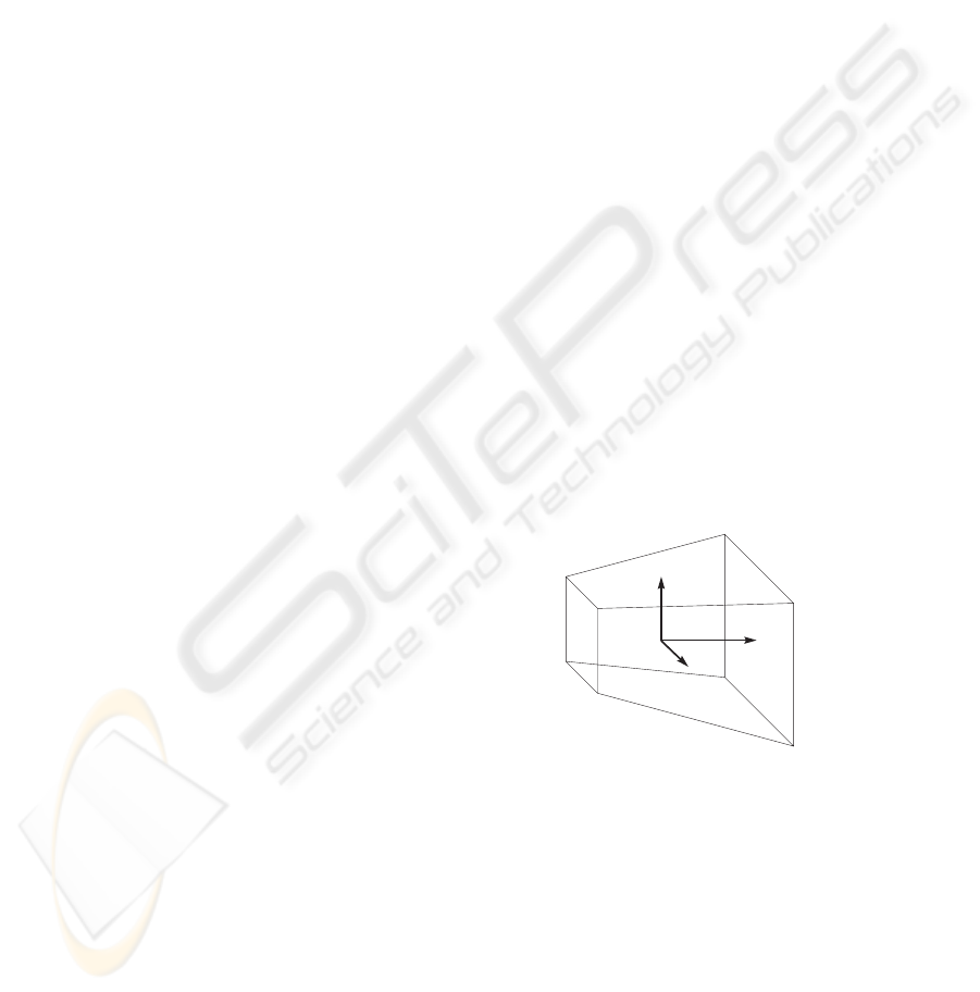
2.2 The Anatomy of a Cell
A cell is a portion of the camera’s viewing frustrum
that results from a recursive subdivision along the u,
v and t parameters. Figure 1 depicts the geometry
of a cell. It has the shape of a truncated pyramid of
quadrangular cross-section, similar to the shape of the
viewing frustrum itself. Four vectors, taken from the
camera’s viewing system, are used to define the spa-
tial extent of a cell. These vectors are:
The vector o This is the location of the camera in the
world coordinate system.
The vectors p
u
and p
v
They represent the horizon-
tal and vertical direction along the image plane.
The length of these vectors gives the width and
height, respectively, of a pixel in the image plane.
The vector p
t
It is the vector from the camera’s
viewpoint and orthogonal to the image plane. The
length of this vector gives the distance from the
viewpoint to the image plane.
The vectors p
u
, p
v
and p
t
define a left-handed per-
spective viewing system. The position of any point x
inside the cell is given by the following inverse per-
spective transformation:
x = o +(up
u
+ vp
v
+ p
t
)t
= o + utp
u
+ vtp
v
+ tp
t
. (3)
t
0
u
e
p
u
t
0
v
e
p
v
t
e
(u
0
p
u
+ v
0
p
v
+ p
t
)
Figure 1: The geometry of a cell. The vectors show the
three medial axes of the cell.
The spatial extent of a cell is obtained from the
above by having the u, v and t parameters vary over
appropriate intervals [ u
a
,u
b
], [ v
a
,v
b
] and [ t
a
,t
b
].
We must consider how to compute the rAA represen-
tation
ˆ
x of this spatial extent. To do so a change of
variables must first be performed. The rAA variable
ˆu = u
0
+ u
e
e
u
will span the same interval [ u
a
,u
b
]
as u does if we have:
u
0
=(u
b
+ u
a
)/2, (4a)
u
e
=(u
b
− u
a
)/2. (4b)
GRAPP 2006 - COMPUTER GRAPHICS THEORY AND APPLICATIONS
28

Similar results apply for the v and t parameters.
Substituting ˆu, ˆv and
ˆ
t in (3) for u, v and t, we get:
x = o + t
0
u
0
p
u
+ t
0
v
0
p
v
+ t
0
p
t
+ t
0
u
e
e
u
p
u
+ t
0
v
e
e
v
p
v
+ u
0
t
e
e
t
p
u
+ v
0
t
e
e
t
p
v
+ t
e
e
t
p
t
+ t
e
u
e
e
u
e
t
p
u
+ t
e
v
e
e
v
e
t
p
v
.
(5)
The first line of (5) contains only constant terms.
The second and third lines contain linear terms of the
noise symbols e
u
, e
v
and e
t
. The fourth line contains
two non-linear terms e
u
e
t
and e
v
e
t
, which are a con-
sequence of the non-linearity of the perspective trans-
formation. Since a rAA representation cannot accom-
modate such non-linear terms they are replaced by the
independent noise terms e
k
1
, e
k
2
and e
k
3
for each of
the three cartesian coordinates of
ˆ
x. The rAA vector
ˆ
x is finally given by:
ˆ
x = o + t
0
(u
0
p
u
+ v
0
p
v
+ p
t
)
+ t
0
u
e
p
u
e
u
+ t
0
v
e
p
v
e
v
+ t
e
(u
0
p
u
+ v
0
p
v
+ p
t
)e
t
+[
x
k
1
e
k
1
x
k
2
e
k
2
x
k
3
e
k
3
]
T
,
(6)
with
x
k
i
= |t
e
u
e
p
u
i
| + |t
e
v
e
p
v
i
|,i=1, 2, 3. (7)
A consequence of the non-linearity of the perspec-
tive projection and its subsequent approximation with
rAA is that the region spanned by
ˆ
x is going to be
larger than the spatial extent of the cell. Figure 2
shows the geometry of a cell and the region spanned
by its rAA representation in profile. Because the rAA
representation has been linearised, its spatial extent
is a prism rather than a truncated pyramid. This has
further consequences in that the evaluation of f(
ˆ
x)
is going to include information from the regions of
the prism outside the cell and will, therefore, lead to
range estimates that are larger than necessary. The
linearisation error is more pronounced for cells that
exist early in the subdivision process. As subdivision
continues and the cells become progressively smaller,
their geometry becomes more like that of a prism and
the discrepancy with the geometry of
ˆ
x decreases
2
.
The subdivision of a cell proceeds by first choos-
ing one of the three perspective projection parameters
u, v or t and splitting the cell in half along that para-
meter. This scheme leads to a k-d tree of cells where
the sequence of dimensional splits is only determined
at run time. The choice of which parameter to split
along is based on the average width, height and depth
2
This can be demonstrated by the fact that the terms t
e
u
e
and t
e
v
e
in (5) decrease more rapidly than any of the linear
terms u
e
, v
e
and t
e
of the same equation as the latter con-
verge to zero.
Figure 2: The outline of a cell (solid line) and the outline of
its rAA representation (dashed line) shown in profile. The
rAA representation is a prism that forms a tight enclosure
of the cell.
of the cell:
¯w
u
=2t
0
u
e
p
u
, (8a)
¯w
v
=2t
0
v
e
p
v
, (8b)
¯w
t
=2t
e
u
0
p
u
+ v
0
p
v
+ p
t
. (8c)
If, say, ¯w
u
is the largest of these three measures,
the cell is split along the u parameter. The two child
cells will have their u parameters ranging inside the
intervals [ u
a
,u
0
] and [ u
0
,u
b
], where [ u
a
,u
b
] was
the interval spanned by u in the mother cell. In prac-
tice, the factors of 2 in (8) can be ignored without
changing the outcome of the subdivision. This subdi-
vision strategy ensures that, after a few iterations, all
the cells will have an evenly distributed shape, even
when the initial cell is very long and thin.
2.3 The Process of Cell Subdivision
Cell subdivision is implemented in an iterative man-
ner rather than using a recursive procedure. The cells
are kept sorted in a priority queue based on their level
of subdivision. A cell has priority over another if it
has undergone less subdivision. For cells at the same
subdivision level, the one that is closer to the camera
will have priority. The algorithm starts by placing the
initial cell, which corresponds to the complete view-
ing frustrum, on the priority queue. At the start of
every new iteration, a cell is removed from the head
of the queue. If the extent of the cell’s projection on
the image plane is larger than the extent of a pixel, the
cell is subdivided and its two children are examined.
In the opposite case, the cell is considered a leaf cell
and is discarded after being rendered. The two condi-
tions that indicate whether a cell should be subdivided
are:
u
b
− u
a
> 1, (9a)
v
b
− v
a
> 1. (9b)
The values on the right hand sides of (9) are a con-
sequence of the definition of p
u
and p
v
in Section 2.2,
which cause all pixels to have a unit width and height.
A PROGRESSIVE REFINEMENT APPROACH FOR THE VISUALISATION OF IMPLICIT SURFACES
29

The sequence of events after a cell has been sub-
divided depends on which of the parameters u, v or
t was used to perform the subdivision. If the subdi-
vision occurred along t, there will be two child cells
with one in front of the other and totally occluding
it. The front cell is first checked for the condition
0 ∈ f(
ˆ
x). If the condition holds, the cell is pushed
into the priority queue and the back cell is ignored.
If the condition does not hold, the back cell is also
checked for the same condition. The difference now
is that, if 0 ∈ f(
ˆ
x) for the back cell, a new cell must
be searched by marching along the t direction. The
first cell scanned, at the same subdivision level of the
front and back cells, for which 0 ∈ f(
ˆ
x) holds is
the one that is pushed into the priority queue. On the
other hand, if the subdivision occurred along the u or
v directions, there will be two child cells that sit side
by side relative to the camera without occluding each
other. Both cells are processed in the same way. If,
for any of the two cells, 0 ∈ f(
ˆ
x) holds, that cell is
placed on the priority queue, otherwise a farther cell
must be searched by marching forward in depth.
Figure 3: Scanning along the depth subdivision tree. Cells
represented by black nodes may intersect with the surface.
Cells represented by white nodes do not. The solid arrows
show progression by depth-first order. The dotted arrows
show progression by breadth-first order.
The process of marching forward from a cell along
the depth direction t tries to find a new cell that has a
possibility of intersecting the implicit surface by veri-
fying the condition 0 ∈ f(
ˆ
x). The process is invoked
when the starting cell has been determined not to ver-
ify the same condition. The reason for having this
scanning in depth is because cells that do not intersect
with the surface must be discarded. Only cells that
verify 0 ∈ f(
ˆ
x) are allowed into the priority queue
for further processing. Figure 3 shows an example of
this marching process. The scanning is performed by
following a depth-first ordering relative to the tree that
results from subdividing in t. The scanning sequence
skips over the children of cells for which 0 ∈ f(
ˆ
x).
The possibility of scanning in breadth-first order, by
marching along all the cells at the same level of sub-
division, is not recommended because in deeply sub-
divided trees a very high number of cells would have
to be tested.
As mentioned before, when subdivision is per-
formed along t, the back cell is ignored whenever the
front cell verifies 0 ∈ f(
ˆ
x). This does not mean, how-
ever, that the volume occupied by this back cell will
be totally discarded from further consideration. The
front cell may happen to be subdivided during subse-
quent iterations of the algorithm and portions of the
volume occupied by the back cell may then be revis-
ited by the depth marching procedure.
2.4 Rendering a Cell
The shading value of a cell is obtained by evaluating
the shading function at the centre of the cell. The cen-
tral point x
0
for the cell is determined from (6) to be:
x
0
= o + t
0
(u
0
p
u
+ v
0
p
v
+ p
t
). (10)
During rendering, the shading value of a cell is as-
signed to all the pixels that are contained within its
image plane projection. The centre of a pixel (i, j)
occupies the coordinates c
ij
=(i +1/2,j +1/2)
on the image plane. All the pixels that verify c
ij
∈
[u
a
,u
b
] × [v
a
,v
b
] for the cell being rendered will
be assigned its shading value. Any previous shad-
ing values stored in these pixels will be overwritten.
This process happens after cell subdivision and before
the newly subdivided cells are placed on the priority
queue. The subdivided cells will overwrite the shad-
ing value of their mother cell on the image buffer. The
same process also takes place for leaf cells before they
are discarded. In this way, the image buffer always
contains the best possible representation of the image
at the start of every new iteration.
2.5 Specifying a Region of Interest
A user can interactively influence the rendering al-
gorithm by drawing a rectangular region of interest
(ROI) over the image. The algorithm will then refine
the image only inside the specified region. This is
accomplished by creating a secondary priority queue
that stores the cells that are relevant to the ROI.
When the user finishes drawing the region, the pri-
mary queue is scanned and all cells whose image pro-
jection intersects with the rectangle corresponding to
that ROI are transferred to the secondary queue. The
algorithm then proceeds as explained in Section 2.3
with the difference that the secondary queue is now
being used. Once this queue becomes empty, the por-
tion of the image inside the ROI is fully rendered
and the algorithm returns to subdividing the cells that
were left in the primary queue. It is also possible to
cancel the ROI at any time by flushing any cells still
in the secondary queue back to the primary queue.
GRAPP 2006 - COMPUTER GRAPHICS THEORY AND APPLICATIONS
30
2.6 Some Implementation Remarks
The best implementation strategy for our rendering
method is to have an application that runs two threads
concurrently: a subdivision thread and a rendering
thread. The rendering thread is responsible for period-
ically updating the graphical output of the application
with the latest results from the subdivision thread. A
timer is used to keep a constant frame refresh rate.
Except for the periodical invocation of the timer han-
dler routine, the rendering thread remains in a sleep
state so that the subdivision thread can use all the CPU
resources.
3 RESULTS
Figure 5 at the end of the paper shows four snap-
shots taken during the progressive refinement render-
ing of an implicit sphere modulated with a Perlin pro-
cedural noise function (Perlin, 2002). The last snap-
shot shows the final rendering of the surface. The
large scale features of the surface become settled quite
early and the latter stages of the refinement are mostly
concerned with resolving small scale details.
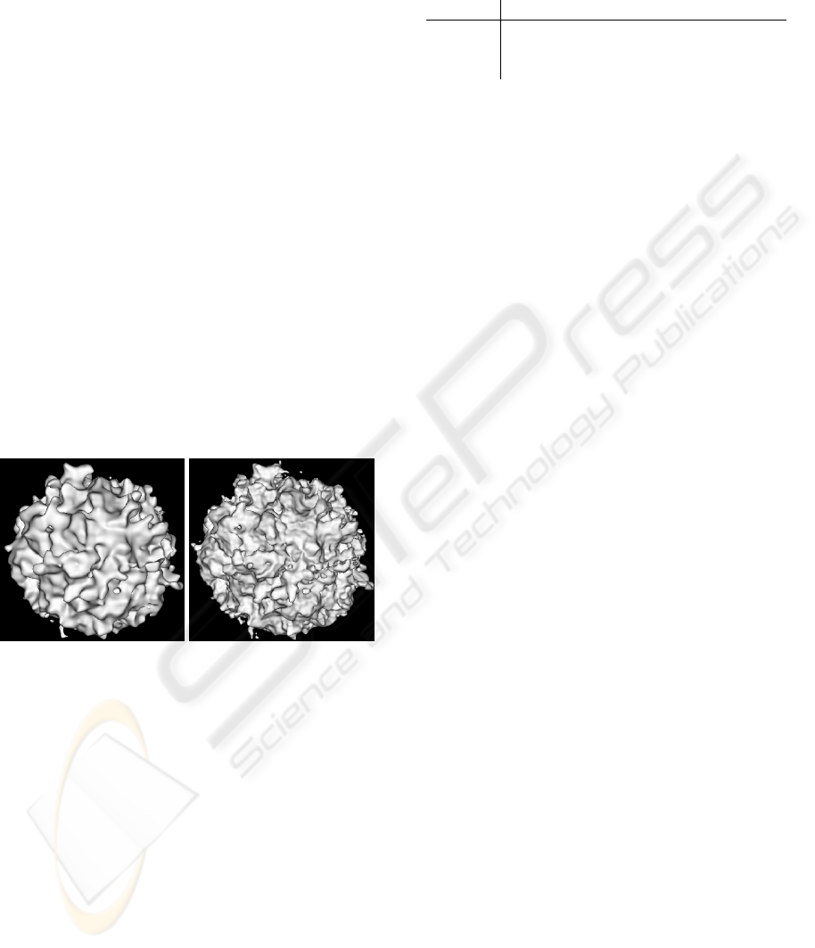
Figure 4: An implicit surface with two layers (left) and three
layers (right) of a Perlin noise function.
Figure 4 shows an implicit sphere modulated with
two and three layers of the Perlin noise function. Ta-
ble 1 shows the total number of iterations and the
computation time for the surfaces that were rendered
in Figures 4 and 5. The table also shows the computa-
tion time for ray casting the same surfaces by shoot-
ing a single ray through the centre of each pixel. The
results in Table 1 were obtained on a laptop with a
Pentium 4 1.8 GHz processor and 1 Gbyte of mem-
ory. The number of iterations required to complete
the progressive rendering algorithm is largely inde-
pendent of the complexity of each surface. It depends
only on the image resolution and on the percentage of
the image that is covered by the projected surface.
As estimated by the results in Table 1, preview-
ing by progressive refinement is approximately three
times faster than previewing by ray casting without
Table 1: Rendering statistics for an implicit sphere with sev-
eral layers of Perlin noise.
Layers Iterations T ime Raycasting
1 350759 27.8s 1m10.4s
2
349465 1m16.8s 4m16.7s
3
359659 3m01.5s 8m51.7s
anti-aliasing. It should be added that these numbers
do not entirely reflect the reality of the situation be-
cause, as demonstrated in the example of Figure 5,
progressive refinement previewing already gives an
accurate rendering of the surface at early stages of re-
finement. From a perceptual point of view, therefore,
the difference between the two previewing techniques
is greater than what is shown in Table 1.
Figure 6 shows two snapshots of a progressive re-
finement rendering where a region of interest is ac-
tive. The surface being rendered is the same two layer
Perlin noise surface that was shown in Figure 4. The
rectangular ROI is defined on the lower right corner
of the image. The portion of the surface that projects
inside the ROI is given priority during progressive re-
finement.
4 CONCLUSIONS
The rendering method, here presented, offers the pos-
sibility of visualising implicit surfaces with progres-
sive refinement. The main features of a surface be-
come visible early in the rendering process, which
makes this method ideal as a previewing tool dur-
ing the editing stages of an implicit surface mod-
eler. In comparison, a meshing method would gen-
erate expensive high resolution preview meshes for
the more complex surfaces while a ray caster would
be slower and without the progressive refinement fea-
ture. Our rendering method, however, does not im-
plement anti-aliasing and cannot compete with an
anti-aliased ray caster as a production tool. Produc-
tion quality renderings of some of the surfaces shown
in this paper are typically done overnight, a fact which
further justifies the need for a previewing tool.
It would have been straightforward to incorporate
anti-aliasing into our rendering method by allowing
cells to be subdivided down to sub-pixel size and then
applying a low-pass filter to reconstruct the pixel sam-
ples. There is, however, one issue that prevents the
use of our method as a production tool and which
makes this implementation effort not worth the while.
As explained in Section 2.1, the computation of range
estimates with affine arithmetic is always conserva-
tive. This conservativeness implies that some cells
a small distance away from the surface may be in-
correctly flagged as intersecting with it. As a conse-
A PROGRESSIVE REFINEMENT APPROACH FOR THE VISUALISATION OF IMPLICIT SURFACES
31

quence, some portions of the surface may appear di-
lated after rendering. The surface offset error is in the
same order as the size of a pixel. This artifact can be
tolerated during previewing but is not acceptable for
production quality renderings.
We intend in the future to apply our progressive re-
finement previewing strategy not only to procedural
fractal planets in implicit form but also to implicit sur-
faces that interpolate scattered data points.
REFERENCES
Bergman, L., Fuchs, H., Grant, E., and Spach, S. (1986).
Image rendering by adaptive refinement. In Evans,
D. C. and Athay, R. J., editors, Computer Graphics
(SIGGRAPH ’86 Proceedings), pages 29–37.
Bloomenthal, J. (1988). Polygonisation of implicit surfaces.
Computer Aided Geometric Design, 5:341–355.
Cohen, M. F., Chen, S. E., Wallace, J. R., and Greenberg,
D. P. (1988). A progressive refinement approach to
fast radiosity image generation. In Dill, J., editor,
Computer Graphics (SIGGRAPH ’88 Proceedings),
pages 75–84.
Comba, J. L. D. and Stolfi, J. (1993). Affine arithmetic
and its applications to computer graphics. In Proc.
VI Brazilian Symposium on Computer Graphics and
Image Processing (SIBGRAPI ’93), pages 9–18.
Cook, R. L. (1989). Stochastic sampling and distributed
ray tracing. In Glassner, A. S., editor, An Introduction
to Ray Tracing, chapter 5, pages 161–199. Academic
Press.
de Figueiredo, L. H. (1996). Surface intersection using
affine arithmetic. In Davis, W. A. and Bartels, R., ed-
itors, Graphics Interface (GI ’96), pages 168–175.
de Figueiredo, L. H. and Stolfi, J. (1996). Adaptive enu-
meration of implicit surfaces with affine arithmetic.
Computer Graphics Forum, 15(5):287–296.
de Figueiredo, L. H., Stolfi, J., and Velho, L. (2003). Ap-
proximating parametric curves with strip trees us-
ing affine arithmetic. Computer Graphics Forum,
22(2):171–171.
Desbrun, M. and Gascuel, M. (1995). Animating soft sub-
stances with implicit surfaces. In Cook, R., editor,
Computer Graphics (SIGGRAPH ’95 Proceedings),
pages 287–290.
Ebert, D. S., Musgrave, F. K., Peachey, D., Perlin, K., and
Worley, S. (2003). Texturing & Modeling: A Proce-
dural Approach. Morgan Kaufmann Publishers Inc.,
third edition.
Farrugia, J. P. and Peroche, B. (2004). A progressive ren-
dering algorithm using an adaptive perceptually based
image metric. Computer Graphics Forum, 23(3):605–
614.
Foster, N. and Fedkiw, R. (2001). Practical animation of liq-
uids. In Pocock, L., editor, Computer Graphics (SIG-
GRAPH ’01 Proceedings), pages 23–30.
Gamito, M. N. and Maddock, S. C. (2005). Ray cast-
ing implicit procedural noises with reduced affine
arithmetic. Memorandum CS – 05 – 04, Dept.
of Comp. Science, The University of Sheffield.
http://www.dcs.shef.ac.uk/
∼mag/CS0504.pdf.
Guo, B. (1998). Progressive radiance evaluation using di-
rectional coherence maps. In Cohen, M., editor, Com-
puter Graphics (ACM SIGGRAPH ’98 Proceedings),
pages 255–266.
Heidrich, W. and Seidel, H.-P. (1998). Ray-tracing proce-
dural displacement shaders. In Davis, W., Booth, K.,
and Fournier, A., editors, Graphics Interface (GI ’98),
pages 8–16.
Heidrich, W., Slusallik, P., and Seidel, H. (1998). Sam-
pling procedural shaders using affine arithmetic. ACM
Transactions on Graphics, 17(3):158–176.
Hin, A. J. S., Boender, E., and Post, F. H. (1989). Vi-
sualization of 3D scalar fields using ray casting. In
Eurographics Workshop on Visualization in Scientific
Computing.
Junior, A., de Figueiredo, L., and Gattas, M. (1999). In-
terval methods for raycasting implicit surfaces with
affine arithmetic. In Proc. XII Brazilian Symposium
on Computer Graphics and Image Processing (SIB-
GRAPI ’99), pages 1–7.
Kolb, C. E. (1992). Rayshade user’s guide and reference
manual. Draft 0.4.
Laur, D. and Hanrahan, P. (1991). Hierarchical splatting: A
progressive refinement algorithm for volume render-
ing. In Sederberg, T. W., editor, Computer Graphics
(SIGGRAPH ’91 Proceedings), pages 285–288.
Lippert, L. and Gross, M. H. (1995). Fast wavelet based vol-
ume rendering by accumulation of transparent texture
maps. Computer Graphics Forum, 14(3):431–444.
Lorensen, W. E. and Cline, H. E. (1987). Marching cubes:
A high resolution 3D surface construction algorithm.
In Stone, M. C., editor, Computer Graphics (SIG-
GRAPH ’87 Proceedings), pages 163–169.
Mitchell, D. P. (1990). Robust ray intersection with interval
arithmetic. In MacKay, S. and Kidd, E. M., editors,
Graphics Interface (GI ’90), pages 68–74.
Moore, R. (1966). Interval Arithmetic. Prentice-Hall, En-
glewood Cliffs (NJ), USA.
Perlin, K. (2002). Improving noise. ACM Transactions on
Graphics, 21(3):681–682.
Roth, S. D. (1982). Ray casting for modeling solids. Com-
puter Graphics and Image Processing, 18(2):109–
144.
Velho, L. (1996). Simple and efficient polygonization of
implicit surfaces. Journal of Graphics Tools, 1(2):5–
24.
Whitaker, R. T. (1998). A level-set approach to 3D recon-
struction from range data. Int. J. Computer Vision,
29:203–231.
GRAPP 2006 - COMPUTER GRAPHICS THEORY AND APPLICATIONS
32
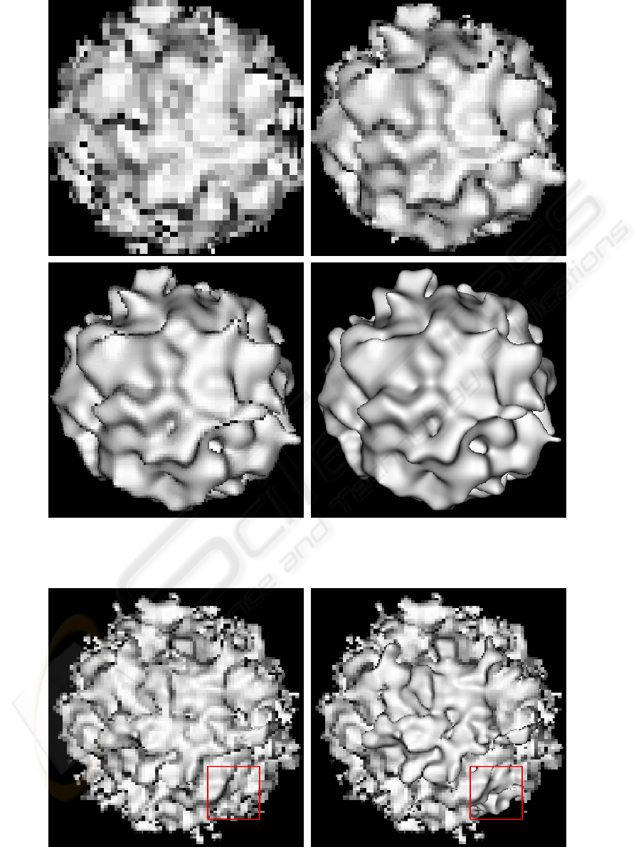
Figure 5: From left to right, top to bottom, snapshots taken during the progressive refinement rendering of a procedural noise
function. The snapshots were taken after 5000, 10000, 28000 and 350759 iterations, respectively. The wall clock times at
each snapshot are 1.02s, 1.98s, 4.18s and 27.80s, respectively.
Figure 6: Progressive refinement rendering with an active region of interest shown as a red frame. Once rendering is complete
inside the region, refinement continues on the rest of the image.
A PROGRESSIVE REFINEMENT APPROACH FOR THE VISUALISATION OF IMPLICIT SURFACES
33
