A NEW NON-UNIFORM LOOP SCHEME

Sandrine Lanquetin, Marc Neveu

LE2I, UMR CNRS 5158, UFR des Sciences et Techniques,

Université de Bourgogne, BP 47870

21078 DIJON Cedex, France

Keywords: Adaptive subdivision, non uniform scheme, Loop scheme.

Abstract: In this paper, we introduce a new non-uniform Loop scheme. It refines selected areas which are chosen

manually or automatically according to the precision of the control mesh compared to the limit surface. Our

algorithm avoids cracks and generates a progressive mesh with a difference of at most one subdivision level

between two adjacent faces. As adaptive subdivision is repeated, subdivision depth changes gradually from

one area of the surface to another area. Moreover generated meshes remain a regular valence. Results

obtained from our scheme are compared to those of the T-algorithm and the incremental algorithm.

1 INTRODUCTION

Subdivision surfaces were introduced in 1978 by

Catmull-Clark (Catmull et al., 1978) and Doo-Sabin

(Doo et al., 1978) as an extension of the Chaikin

algorithm (Chaikin, 1974)]. These surfaces are

widely used in character animation (such as Geri's

Game © or Finding Nemo ©) to smooth models.

Indeed, from a coarse mesh, successive refinements

give finer meshes. A sequence of subdivided meshes

converges towards a smooth surface called limit

surface. Since the beginning of subdivision surfaces

in 1978, many subdivision schemes were proposed.

Some are approximating and others are interpolating

(i.e. control vertices of successive meshes belong to

the limit surface). We focus on Loop subdivision

(Loop, 1987) for this research. This scheme is

approximating and can only be applied on triangular

meshes.

Most of schemes were first uniform. In uniform

schemes, the subdivision rules are the same for the

whole input model. For example, the Loop scheme

splits each face of the input mesh into four. The

number of faces quickly increases whereas there is

generally no need to smooth the model everywhere.

Indeed, subdivisions do not bring much geometric

modification into flat areas; faces which are not

visible do not need many subdivisions. Other

geometric criteria can be used such as accuracy or

curvature. Or more simply, users can manually

choose faces or vertices to be subdivided.

Non uniform subdivision (also called adaptive

subdivision) can be decomposed into two parts.

First, an area to be subdivided has to be chosen by

different ways such as in (Amresh et al., 2003),

(Dyn et al., 1990), (Meyer et al., 2002), (Zorin et al.,

1998). Secondly, topological rules have to be

determined such as in (Amresh et al., 2003), (Pakdel

et al., 2004), (Seeger et al., 2001), (Zorin et al.,

1998). These rules aim to generate a new mesh

without the cracks that can be caused by a difference

between the subdivision levels of two adjacent faces.

In the case of Loop’s triangular scheme, rules have

to preserve triangular faces.

In this paper, we focus on the topological problem.

Some algorithms already deal with this subject.

Thus, the algorithm of Seeger et al. splits adjacent

faces into two if they present a crack and into four

otherwise (Seeger et al., 2001). Amresh et al.

similarly propose to split faces into two, three or

four faces according to the number of cracks created

by the face subdivision (Amresh et al., 2003). From

these algorithms, Pakdel and Samavati extend the

rules to produce a smooth surface with visually

pleasing connectivity (Pakdel et al., 2004).

Our contribution consists in new topological rules

for non-uniform Loop subdivision. The algorithm

we propose takes advantages of the above mentioned

algorithms. Indeed, our algorithm produces meshes

with progressive changes between faces of different

subdivision level but without subdividing a too large

134

Lanquetin S. and Neveu M. (2006).

A NEW NON-UNIFORM LOOP SCHEME.

In Proceedings of the First International Conference on Computer Graphics Theory and Applications, pages 134-141

DOI: 10.5220/0001350301340141

 SciTePress

surrounding area. Obviously, the more extended the

area is, the higher the number of generated faces is.

The paper is organized as follows. Section 2 is an

overview of uniform and non-uniform Loop

schemes. In section 3, we explain disadvantages and

advantages of existing adaptive schemes and how

our algorithm works. Finally, we compare our

algorithm with the others on some examples in

section 4.

2 BACKGROUND

2.1 Loop Scheme

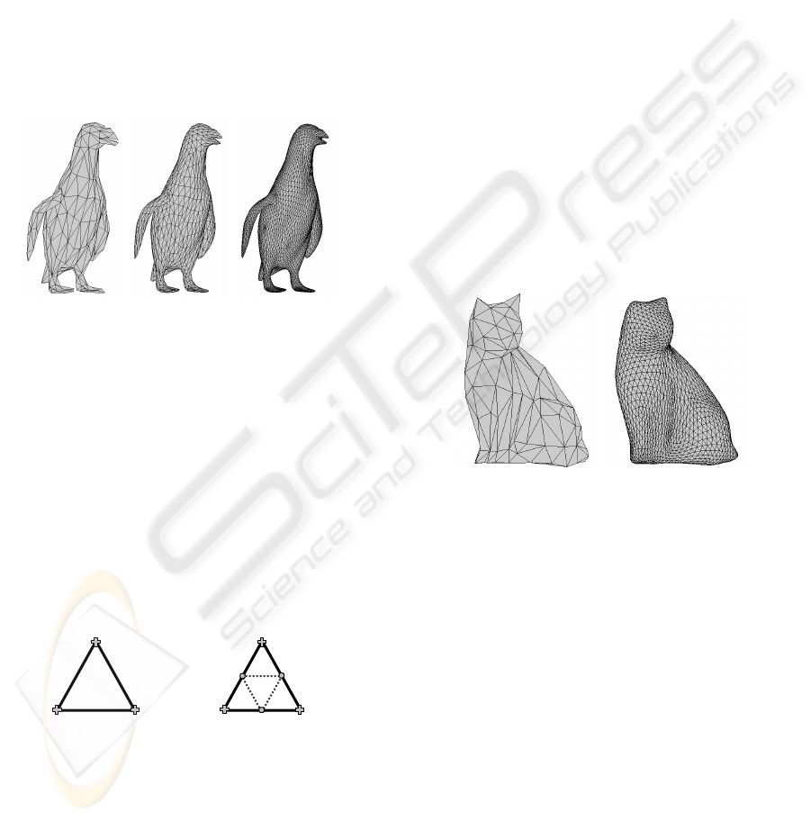
Figure 1: From left to right: the initial penguin mesh and

two successive levels of Loop subdivision.

Subdivision surfaces are defined by an initial control

mesh and a set of refinement rules. The application

of refinement rules generates a sequence of

increasingly fine control meshes. Control meshes are

often referred to as polygonal meshes or

polyhedrons. The sequence of control meshes

converges to a smooth surface called the limit

surface. There are two sorts of subdivision schemes:

schemes which rely on interpolation (e.g. Butterfly

scheme (Dyn et al., 1990)) or approximation (e.g.

Catmull-Clark (Catmull et al., 1978), Doo-Sabin

(Doo et al., 1978), Loop (Loop, 1987) schemes…).

Figure 2: Left, an initial face. Right, the 4 new faces.

A particularity of approximation schemes is that

control meshes approach the limit surface at each

step of refinement. Figure 1 shows three successive

meshes obtained by applying Loop scheme.

The Loop scheme generalizes quadratic triangular

B-splines and the obtained limit surface is a quartic

Box-spline. This scheme is based on face splitting:

each face of the control mesh at refinement level

is subdivided into four new triangular faces at level

. This first step is illustrated in Figure 2.

Consider a face: new vertices -named odd vertices-

are inserted in the middle of each edge, and those of

the initial face are named even vertices. In the

second step, all vertices are displaced by computing

a weighted average of the vertex and its

neighbouring vertices. These averages can be

substituted by applying different masks according to

vertex properties: even/odd, interior/boundary

2.2 Adaptive Subdivision

When the same rules are applied on the whole input

mesh, the number of faces quickly increases. Indeed,

for Loop scheme, a face produces four faces after

one subdivision,

4 after 2 subdivisions and 4

after

n subdivisions. Thus, the cat model introduced in

Figure 3 has 224 faces at the initial level (Figure 3,

left) and 3584 after two subdivisions (Figure 3,

right).

Figure 3: Left: the initial cat model. Right: the cat mesh

after two subdivisions.

However, there is often no need to smooth the

model in the same way everywhere according to

surface properties or specific applications. For

example, if a surface is flat, there is no need to

subdivide it anymore. Indeed, in this case, new

generated faces do not improve quality of the mesh.

In a similar way, an area of the mesh which already

looks smooth will not change anymore after new

subdivision levels. Another idea is to smooth only

visible parts of the mesh. The mesh can also be

subdivided only where the mesh does not

approximate the limit surface with enough precision.

Thus, only some areas of the input mesh can be

subdivided to generate an optimal mesh with a

smaller number of faces.

When the surface is not entirely subdivided,

cracks appear between faces with different

subdivision levels as shown in Figure 4.

A NEW NON-UNIFORM LOOP SCHEME

135

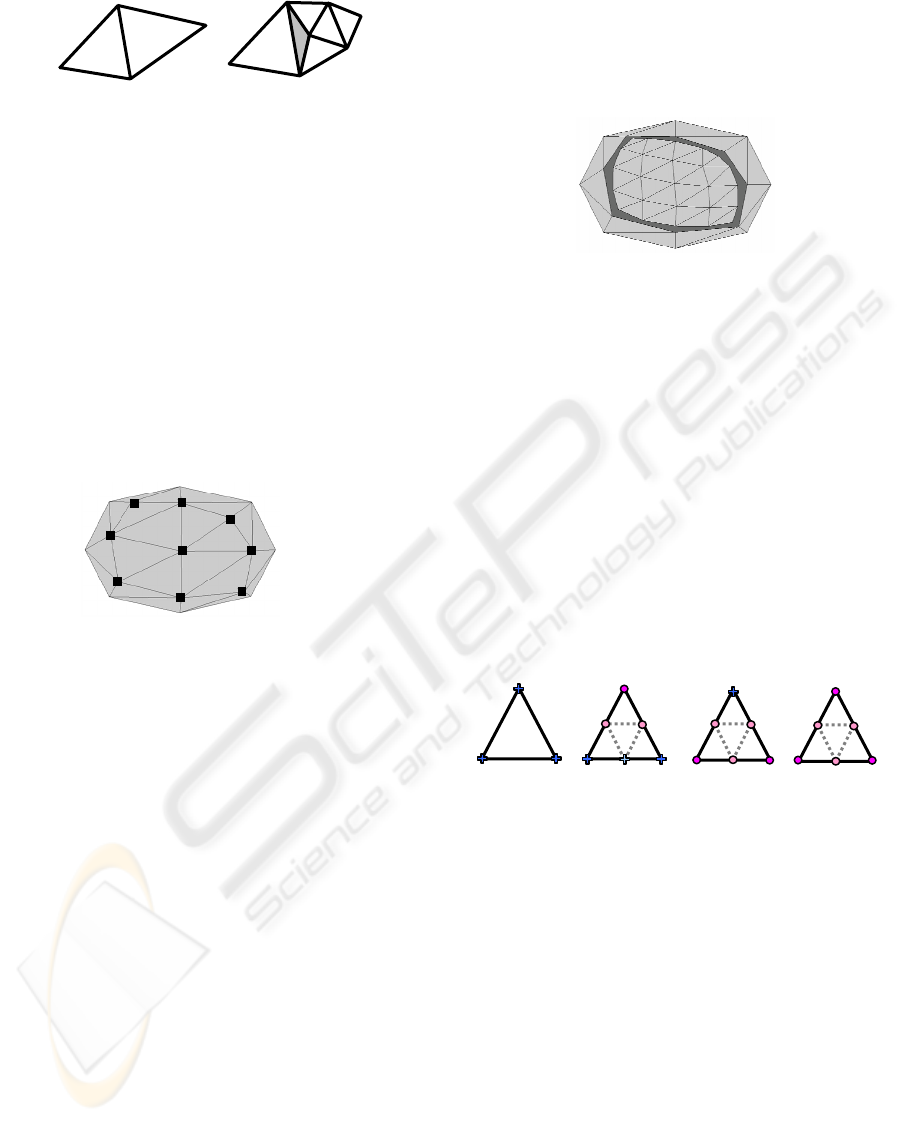
Figure 4: Left: two adjacent faces of the mesh. Right: one

face is subdivided and not the other, the crack between the

faces is represented in grey.

To avoid cracks, topological rules have to be

modified. As rules are different according to

subdivision areas, this kind of scheme is called non-

uniform or adaptive.

Selection criteria. The area to be subdivided can be

selected by different ways.

First, users can manually choose faces or vertices

they want to subdivide. This choice can be done

arbitrarily or according to the required details in a

specific area. Figure 5 illustrates a mesh with

selected vertices to be subdivided in dark grey.

Figure 5: Example of manual selection.

Another criterion for adaptive subdivision, which

is often used, is the surface curvature. In this case,

the model is refined where the model has high

curvatures. Thus, Dyn et al. (Dyn et al., 2000)

automatically determine the area to subdivide

according to the discrete curvature and apply it on

the butterfly scheme. Meyer et al. compute Gaussian

curvature from its sums of Voronoi area (Meyer et

al., 2002). Others works are based on

approximations of the surface curvatures which are

easier to compute. Xu and Kondo (Xu et al., 1999)

and Amresh et al. (Amresh et al., 2003) use the

dihedral angle criterion (the angle between normals

of adjacent faces). Müller and Havemann (Müller et

al., 2000) propose another approximation of the

surface curvature by computing, for each vertex of

the mesh, the normal cone (the angle between

normals of adjacent faces to a vertex). Another

criterion can be the accuracy of the control mesh

compared to the limit surface (Lanquetin, 2004). In

(Isenberg et al., 2003), Isenberg et al. generalizes

adaptive subdivision algorithms by introducing an

application-dependent Degree of Interest function.

Topological rules. To avoid cracks which appear

when the surface is not entirely subdivided, there

exist different methods. Figure 6 shows these cracks

on a mesh for which only faces selected in Figure 5

are subdivided with Loop scheme.

Figure 6: Example of cracks.

Various topological rules were already proposed in

(Amresh et al., 2003), (Lanquetin, 2004), (Pakdel et

al., 2004), (Seeger et al., 2001) and (Zorin et al.,

1998). We will describe them in section 3.

3 TOPOLOGICAL RULES

3.1 Existing Topological Rules

A simple method presented in (Lanquetin, 2004) and

used in (Lanquetin et al., 2004) generates a

minimum number of faces. The surface is only

subdivided where the distance is greater than a given

threshold.

Figure 7: Different cases of subdivision in the simple

adaptive subdivision.

Let us first define the terms used to explain how

faces are subdivided in this adaptive subdivision: a

vertex which is not displaced is called static and a

vertex which is displaced is called mobile. Faces are

classified into 4 categories according to the number

of mobile vertices. Mobile vertices are depicted by

circles in Figure 7. When all vertices are static, the

face is not subdivided (Figure 7.a.). Figure 7.b.

illustrates the case where only one vertex is mobile;

only two among the three new vertices are then

mobile in order to avoid cracks. When there are two

mobile vertices, face subdivision is almost normal

except for the fact that one of the old vertices is

static (Figure 7.c.). Finally when all vertices are

mobile, subdivision is carried out in a normal way

(Figure 7.d.).

c. d. b.

GRAPP 2006 - COMPUTER GRAPHICS THEORY AND APPLICATIONS

136

This scheme generates a minimum number of

faces because faces which have 3 static points are no

more subdivided. This adaptive subdivision scheme

avoids cracks but the resulting mesh is not

conformal (Figure 9). Indeed, the case shown in

Figure 8 appears between subdivided faces and not.

The edge of the face which is not subdivided

corresponds to two edges of subdivided faces. In

Figure 8, vertices represented by crosses are no more

subdivided and those represented by circles are still

subdivided.

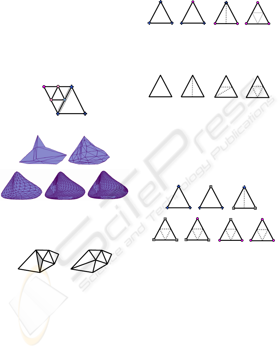
Figure 8: New neighbourhood.

Figure 9: Successive mesh subdivisions with without

proper neighbourhood.

Following methods reconstruct a proper mesh

after successive subdivisions.

Figure 10: Left: one face is subdivided and not the other,

the crack between faces is represents in grey. Right:

bisection of adjacent faces by an edge to avoid cracks.

Zorin et al. (Zorin et al., 1998) and Amresh et al.

(Amresh et al., 2003) remove cracks in subdividing

chosen faces and bisecting adjacent faces by an

edge. The bisection is done in connecting the vertex

with the incomplete structure to the opposite vertex

of the adjacent face as shown in Figure 10.

In Figure 11, mobile vertices are denoted by

circles and others by crosses. In the following, this

scheme will be called T-algorithm.

Figure 11: Topological rules for the T-algorithm.

Seeger et al. (Seeger et al., 2001) focus on the

butterfly scheme. Their algorithm, called red-green

triangulation, splits faces into two, three or four

faces as illustrated in Figure 12.

Figure 12: Different cases of face splitting used in the red-

green algorithm.

Pakdel and Samavati (Pakdel et al., 2004) extend

the method introduced in (Amresh et al., 2003) to

remove cracks after adaptative subdivision. To

maintain a restricted mesh (Zorin et al., 1998) during

subdivision, they select a larger subdivision area

than the specified one. They call their algorithm

incremental algorithm. They introduce progressive

vertices, denoted by squares in Figure 13.

Figure 13: Topological rules for the incremental

algorithm.

Each vertex in the 1-neighbourhood of the

selected area is tagged as progressive. Then,

according to the vertex tag: mobile (circle),

progressive (square) or static (cross), faces are

subdivided as illustrated in Figure 13.

A NEW NON-UNIFORM LOOP SCHEME

137

3.2 Our Topological Rules

Our algorithm takes advantages of both T-algorithm

and incremental algorithm. In the following this

scheme will be called diagonal algorithm. It selects a

larger subdivision area than the T-algorithm but a

smaller one than the incremental algorithm. Faces

selected are normally subdivided. Then, adjacent

faces by an edge are split into four and adjacent

faces by a vertex are split into three as shown in

Figure 14. Vertices to be subdivided are denoted by

circles and others by crosses.

Figure 14: Topological rules for the diagonal algorithm.

In contrast with the T-algorithm, the diagonal

algorithm removes cracks outside the selected area

so that the subdivision is progressive and new

valences are not too high. Indeed, adjacent faces are

at most one subdivision depth apart, so the

connectivity between faces does not abruptly

change. As vertices where trisection is applied once

are no more subdivided, the valence of this vertex no

more increases. This avoids generating too high

valences.

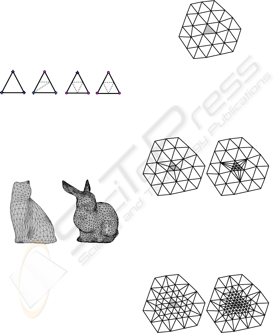
Figure 15: Subdivision of the cat and the bunny models

with the diagonal adaptive algorithm.

Moreover, contrary to incremental algorithm, the

additional selected area is smaller so that the final

mesh has less faces. Indeed the goal of adaptive

subdivision is to generate meshes with less faces.

Meshes obtained on the cat and the bunny models

are shown in Figure 15.

3.3 Successive Subdivisions

Differences between the T-algorithm, the

incremental algorithm and the diagonal algorithm

are now shown on an example. Let the initial mesh

be the mesh drawn in Figure 16 and the selected area

be the face in grey.

Figure 16: The selected face to subdivide is in grey.

The three algorithms will now be applied on the

mesh in Figure 16. Figure 17 shows two subdivision

levels obtained with the T-algorithm. The number

of faces is 43 after one subdivision and 61 after two.

So there are few generated faces. However, at the

second subdivision level, some introduced valences

are extraordinary and become higher and higher with

successive subdivisions.

Figure 17: Two subdivisions of the grey face with the T-

algorithm.

To avoid this problem of high valences, the

incremental algorithm takes a larger area around the

selected faces. Results of one and two subdivisions

are illustrated in Figure 18.

The number of faces is very high from the first

subdivision: 85 at the first subdivision and 159 at the

second. Nevertheless valences are almost regular as

vertex valences are five, six or seven.

Figure 18: Two subdivisions of the grey face with the

incremental algorithm.

GRAPP 2006 - COMPUTER GRAPHICS THEORY AND APPLICATIONS

138

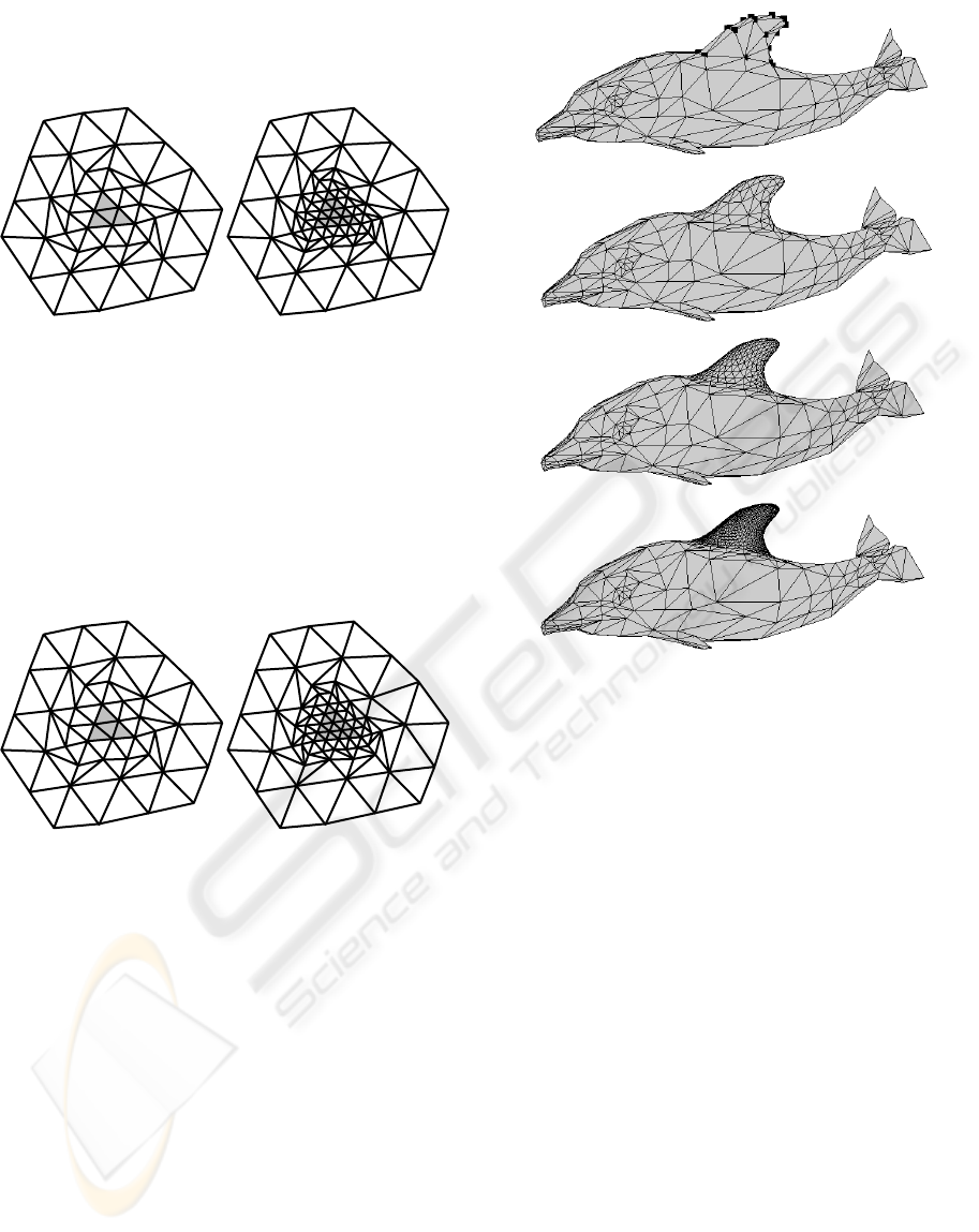
The diagonal algorithm gives an intermediate

number of faces: 67 at the first level and 121 at the

second level as shown in Figure 19.

Figure 19: Twice subdivision of the grey face with the

diagonal algorithm.

Like incremental algorithm, valences are almost

regular: six or seven. Moreover the subdivision

depth between faces is progressive. However, the

diagonal of the trapezium (during trisection) gives a

spiral appearance. To improve this, we can take one

diagonal of the trapezium at a subdivision level and

the other at the next subdivision level as shown in

Figure 20.

Figure 20: Two subdivisions of the grey face with a

variant of the diagonal algorithm.

4 RESULTS AND COMPARISON

In Figure 21, the selected area is the fin of the

dolphin model. Vertices from the faces to subdivide

are tagged by black squares (top). Then, the diagonal

algorithm is applied three times and resulting

meshes are represented in Figure 21.

Figure 21: From top to bottom, three adaptive subdivisions

of the selected dolphin fin.

The cat model automatically subdivided

according to the accuracy of the mesh approximation

in relation to the limit surface with the three

algorithms is shown in Figure 22. The initial cat

model consists in 224 faces (Figure 3). In

Figure 22,

the left mesh obtain with the T-algorithm has 898

faces, the incremental algorithm generates 1444

faces (center) and the diagonal algorithm produces

1226 faces (right).

On the left mesh in

Figure 22, two extraordinary

valences appear but the result is correct. Moreover

incremental algorithm and the diagonal algorithm

give similar results in number of faces.

A NEW NON-UNIFORM LOOP SCHEME

139

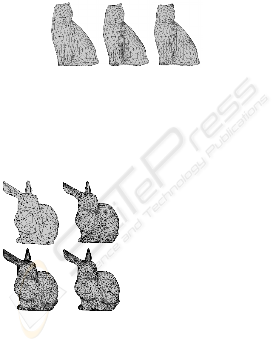
Figure 22: Meshes obtained respectively with the T-algorithm, the incremental algorithm and the diagonal algorithm.

We now compare results of the three algorithms

on a bigger mesh. The initial bunny mesh has 592

faces and we choose a smaller accuracy. In

Figure 23,

meshes are represented as follows. From top to

bottom and from left to right: the initial mesh, the T-

algorithm mesh, the incremental algorithm mesh and

the mesh generated by the diagonal algorithm. The

T-algorithm still gives the smaller mesh with 3094

faces but degenerated valences appear. For the

second time, incremental algorithm and the diagonal

algorithm give correct meshes but this time, the

incremental algorithm creates 5426 faces whereas

the diagonal algorithm generates 4282 faces.

Figure 23: Initial mesh and meshes obtained respectively

with the T-algorithm, the incremental algorithm and the

diagonal algorithm.

5 CONCLUSION

In uniform schemes, the subdivision rules are the

same for the whole input model. As there is often no

need to subdivide the whole mesh, non-uniform

subdivision is used such as the T-algorithm or the

incremental algorithm. The algorithm we introduced

in this paper takes advantages of both the T-

algorithm and the incremental algorithm. It refines

selected areas which are chosen manually or

automatically according to the accuracy of the

control mesh compared to the limit surface.

Subdivision rules avoid cracks and generate a

progressive mesh with at most one subdivision level

between two adjacent faces and proper connectivity.

Moreover valences remain regular on most of the

vertices.

REFERENCES

Amresh A., Farin G. and Razdan A., Adaptive subdivision

schemes for triangular meshes, in Hierarchical and

Geometric Methods in Scientific Visualization, H.H.

G. Farin, and B. Hamann, editors, Editor. 2003. p.

319-327.

Catmull E. and Clark J., Recursively generated B-spline

surfaces on arbitrary topological meshes. Computer

Aided Design, 1978. 9(6): p. 350-355.

Chaikin G. (1974). "An algorithm for High Speed Curve

Generation." CGIP 3, p. 346 - 349.

Doo D. and Sabin M., Behaviour of recursive subdivision

surfaces near extraordinary points. Computer Aided

Design, 1978. 9(6): p. 356-360.

Dyn N., Levin D., and Gregory J.A., A butterfly

subdivision scheme for surface interpolation with

tension control. ACM Transactions on Graphics, 1990.

9: p. 160-169.

Dyn N., Hormann K., Kim S. and Levin D. (2000).

"Optimizing 3D triangulations using discrete curvature

analysis, Oslo." Mathematical Methods for Curves and

Surfaces, p. 135-146.

Isenberg T., Hartmann K. and König H., Interest value

driven adaptive subdivision. In T. Schulze, S.

GRAPP 2006 - COMPUTER GRAPHICS THEORY AND APPLICATIONS

140

Schlechtweg, and V. Hinz, editors, Simulation und

Visualisierung, pages 139–149. SCS European

Publishing House, March 2003.

Lanquetin S., Etude des surfaces de subdivision :

intersection, précision et profondeur de subdivision.

PhD thesis, University of Burgundy, France, 2004.

Lanquetin S. and Neveu M., A priori computation of the

number of surface subdivision levels.Proceedings of

Computer Graphics and Vision (GRAPHICON 2004),

pp. 87-94, September 6-8, 2004, Moscow, Russia.

Loop C., Smooth Subdivision Surfaces Based on

Triangles. Department of Mathematics: Master's

thesis, University of Utah, 1987.

Meyer M., Desbrun M., Schröder P., and Barr A., Discrete

differential-geometry operators for triangulated 2-

manifolds. VisMath, 2002.

Müller K. and Havemann S., Subdivision Surface

Tesselation on the Fly using a Versatile Mesh data

Structure. Eurographics'2000, 2000. 19(3): p. 151-159.

O'Brien, D.A. and D. Manocha, Calculating Intersection

Curve Approximations for Subdivision Surfaces.

2000.

Pakdel H. and Samavati F., Incremental adaptive Loop

subdivision. ICCSA 2004, LNCS 3045, pp. 237-246,

2004.

Seeger S., Hormann K., Häusler G., and Greiner G., A

sub-atomic subdivision approach. In T. Ertl, B. Girod,

G. Greiner, H. Niemann, and H. P. Seidel, editors,

Proceedings of the Vision Modeling and Visualization

Conference 2001 (VMV-01), pages 77–86, Berlin,

November 2001. Aka GmbH.

Xu Z. and Kondo K. (1999). "Adaptive renements in

subdivision surfaces." Eurographics '99, Short papers

and demos, p. 239-242.

Zorin D., Schröder P., and Sweldens W., Interactive

multiresolution mesh editing. SIGGRAPH'98

Proceedings, 1998: p. 259-268.

A NEW NON-UNIFORM LOOP SCHEME

141