ALGORITHMIC SKELETONS FOR BRANCH & BOUND

Michael Poldner

University of M

unster, Department of Information Systems

Leonardo Campus 3, D-48149 M

unster, Germany

Herbert Kuchen

University of M

unster, Department of Information Systems

Leonardo Campus 3, D-48149 M

unster, Germany

Keywords:

Parallel Computing, Algorithmic Skeletons, Branch & Bound, Load Distribution, Termination Detection.

Abstract:

Algorithmic skeletons are predeﬁned components for parallel programming. We will present a skeleton for

branch & bound problems for MIMD machines with distributed memory. This skeleton is based on a dis-

tributed work pool. We discuss two variants, one with supply-driven work distribution and one with demand-

driven work distribution. This approach is compared to a simple branch & bound skeleton with a centralized

work pool, which has been used in a previous version of our skeleton library Muesli. Based on experimental

results for two example applications, namely the n-puzzle and the traveling salesman problem, we show that

the distributed work pool is clearly better and enables good runtimes and in particular scalability. Moreover,

we discuss some implementation aspects such as termination detection as well as overlapping computation

and communication.

1 INTRODUCTION

Today, parallel programming of MIMD machines

with distributed memory is mostly based on message-

passing libraries such as MPI (W. Gropp, 1999; MPI,

2006). The resulting low programming level is error-

prone and time consuming. Thus, many approaches

have been suggested, which provide a higher level

of abstraction and an easier program development.

One such approach is based on so-called algorith-

mic skeletons (Cole, 1989; Cole, 2006), i.e. typical

patterns for parallel programming which are often of-

fered to the user as higher-order functions. By provid-

ing application-speciﬁc parameters to these functions,

the user can adapt an application independent skele-

ton to the considered parallel application. (S)he does

not have to worry about low-level implementation de-

tails such as sending and receiving messages. Since

the skeletons are efﬁciently implemented, the result-

ing parallel application can be almost as efﬁcient as

one based on low-level message passing.

Algorithmic skeletons can be roughly divided

into data parallel and task parallel ones. Data-

parallel skeletons (see e.g. (R. Bisseling, 2005;

G. H. Botorog, 1996; G. H. Botorog, 1998;

H. Kuchen, 1994; Kuchen, 2002; Kuchen, 2004))

process a distributed data structure such as a dis-

tributed array or matrix as a whole, e.g. by applying

a function to every element or by rotating or permut-

ing its elements. Task-parallel skeletons (A. Benoit,

2005; Cole, 2004; Hofstedt, 1998; H. Kuchen,

2002; Kuchen, 2002; Kuchen, 2004; Pelagatti, 2003)

construct a system of processes communicating via

streams of data. Such a system is mostly generated

by nesting typical building blocks such as farms and

pipelines. In the present paper, we will focus on a

particular task-parallel skeleton, namely a branch &

bound skeleton.

Branch & bound (G.L. Nemhauser, 1999) is a

well-known and frequently applied approach to solve

certain optimization problems, among them inte-

ger and mixed-integer linear optimization problems

(G.L. Nemhauser, 1999) and the well-known travel-

ing salesman problem (J.D.C. Little, 1963). Many

practically important but NP-hard planning problems

can be formulated as (mixed) integer optimization

problems, e.g. production planning, crew scheduling,

and vehicle routing. Branch & bound is often the only

practically successful approach to solve these prob-

lems exactly. In the sequel we will assume without

loss of generality that an optimization problem con-

sists of ﬁnding a solution value which minimizes an

objective function while observing a system of con-

straints. The main idea of branch & bound is the fol-

291

Poldner M. and Kuchen H. (2006).

ALGORITHMIC SKELETONS FOR BRANCH & BOUND.

In Proceedings of the First International Conference on Software and Data Technologies, pages 291-300

DOI: 10.5220/0001315002910300

 SciTePress

lowing. A problem is recursively divided into sub-

problems and lower bounds for the optimal solution

of each subproblem are computed. If a solution of

a (sub)problem is found, it is also a solution of the

overall problem. Then, all other subproblems can

be discarded, whose corresponding lower bounds are

greater than the value of the solution. Subproblems

with smaller lower bounds still have to considered re-

cursively.

Only little related work on algorithmic skeletons

for branch & bound can be found in the literature

(E. Alba, 2002; F. Almeida, 2001; I. Dorta, 2003;

Hofstedt, 1998). However, in the corresponding liter-

ature there is no discussion of different designs. The

MaLLBa implementation is based on a master/worker

scheme and it uses a central queue (rather than a heap)

for storing problems. The master distributes problems

to workers and receives their solutions and generated

subproblems. On a shared memory machine this ap-

proach can work well. We will show in the sequel

that a master/worker approach is less suited to handle

branch & bound problems on distributed memory ma-

chines. In a previous version of the Muesli skeleton

library, a branch & bound skeleton with a centralized

work pool has bee used, too (H. Kuchen, 2002). Hof-

stedt outlines a B&B skeleton with a distributed work

pool. Here, work is only shared, if a local work pool

is empty. Thus, worthwhile problems are not propa-

gated quickly and their investigation is concentrated

on a few workers only.

The rest of this paper is structured as follows. In

Section 2, we recall, how branch & bound algorithms

can be used to solve optimization problems. In Sec-

tion 3, we introduce different designs of branch &

bound skeletons in the framework of the skeleton li-

brary Muesli (Kuchen, 2002; Kuchen, 2004; Kuchen,

2006). After describing the simple centralized design

considered in (H. Kuchen, 2002), we will focus on

a design with a distributed work pool. Section 4 con-

tains experimental results demonstrating the strengths

and weaknesses of the different designs. In Section 5,

we conclude and point out future work.

2 BRANCH & BOUND

Branch & bound algorithms are general methods used

for solving difﬁcult combinatorial optimization prob-

lems. In this section, we illustrate the main prin-

ciples of branch & bound algorithms using the 8-

puzzle, a simpliﬁed version of the well-known 15-

puzzle (Quinn, 1994), as example. A branch & bound

algorithm searches the complete solution space of a

given problem for the best solution. Due to the ex-

ponentially increasing number of feasible solutions,

their explicit enumeration is often impossible in prac-

tice. However, the knowledge about the currently best

solution, which is called incumbent, and the use of

bounds for the function to be optimized enables the

algorithm to search parts of the solution space only

implicitly. During the solution process, a pool of yet

unexplored subsets of the solution space, called the

work pool, describes the current status of the search.

Initially there is only one subset, namely the com-

plete solution space, and the best solution found so

far is inﬁnity. The unexplored subsets are repre-

sented as nodes in a dynamically generated search

tree, which initially only contains the root, and each

iteration of the branch & bound algorithm processes

one such node. This tree is called the state-space tree.

Each node in the state-space tree has associated data,

called its description, which can be used to determine,

whether it represents a solution and whether it has any

successors. A branch & bound problem is solved by

applying a small set of basic rules. While the signa-

ture of these rules is always the same, the concrete

formulation of the rules is problem dependent. Start-

ing from a given initial problem, subproblems with

pairwise disjoint state spaces are generated using an

appropriate branching rule. A generated subproblem

can be estimated applying a bounding rule. Using a

selection rule, the subproblem to be branched from

next is chosen from the work pool. Last but not least

subproblems with non-optimal or inadmissible solu-

tions can be eliminated during the computation using

an elimination rule. The sequence of the application

of these rules may vary according to the strategy cho-

sen for selecting the next node to process (J. Clausen,

1999). As an example of the branch and bound tech-

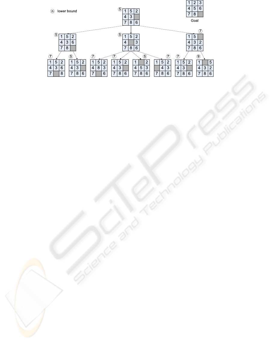
nique, consider the 8-puzzle (Quinn, 1994). Figure 1

illustrates the goal state of the 8-puzzle and the ﬁrst

three levels of the state-space tree.

The 8-puzzle consists of eight tiles, numbered 1

through 8, arranged on a 3 × 3 board. Eight positions

on the board contain exactly one tile and the remain-

ing position is empty. The objective of the puzzle is

to repeatedly ﬁll the hole with a tile adjacent to it in

horizontal or vertical direction, until the tiles are in

row major order. The aim is to solve the puzzle in the

least number of moves.

The branching rule describes, how to split a prob-

lem represented by a given initial board into subprob-

lems represented by the boards resulting after all valid

moves. A minimum number of tile moves needed to

solve the puzzle can be estimated by adding the num-

ber of tile moves made so far to the Manhattan dis-

tance between the current position of each tile and its

goal position. The computation of this lower bound is

described by the bounding rule.

The state-space tree represents all possible boards

that can be reached from the initial board. One way

to solve this puzzle is to pursue a breadth ﬁrst search

or a depth ﬁrst search of the state-space tree until the

ICSOFT 2006 - INTERNATIONAL CONFERENCE ON SOFTWARE AND DATA TECHNOLOGIES

292

Hole

Figure 1: Upper part of the state-space tree corresponding to an instance of the 8-puzzle and its goal board.

sorted board is discovered. However, we can often

reach the goal faster by selecting the node with the

best lower bound to branch from. This selection rule

corresponds to a best-ﬁrst search strategy. Other se-

lection rules such as a variant of depth-ﬁrst search

are discussed in (J. Clausen, 1999; Y. Shinano, 1995;

Y. Shinano, 1997).

Branch & bound algorithms can be parallelized at

a low or at a high level. In case of a low-level paral-

lelization, the sequential algorithm is taken as a start-

ing point and just the computation of the lower bound,

the selection of the subproblem to branch from next,

and/or the application of the elimination rule are per-

formed by several processes in a data parallel way.

The overall behavior of such a parallel algorithm re-

sembles of the sequential algorithm.

In case of a high-level parallelization, the effects

and consequences of the parallelism are not restricted

to a particular part of the algorithm, but inﬂuence the

algorithm as a whole. Several iterations of the main

loop are performed in a task-parallel way, such that

the state-space tree is explored in a different (non-

deterministic!) order than in the sequential algorithm.

3 BRANCH & BOUND

SKELETONS

In this section, we will consider different implemen-

tation and design issues of branch & bound skeletons.

For the most interesting distributed design, several

work distribution strategies are discussed and com-

pared with respect to scalability, overhead, and per-

formance. Moreover, a corresponding termination de-

tection algorithm is presented.

A B&B skeleton is based on one or more branch

& bound algorithms and offers them to the user as

predeﬁned parallel components. Parallel branch &

bound algorithms can be classiﬁed depending on the

organization of the work pool. A central, distributed,

and hybrid organization can be distinguished. In

the MaLLBa project, a central work pool is used

(F. Almeida, 2001; I. Dorta, 2003). Hofstedt (Hofst-

edt, 1998) sketches a distributed scheme, where work

is only delegated, if a local work pool is empty. Shi-

nano et al. (Y. Shinano, 1995; Y. Shinano, 1997)

and Xu et al. (Y. Xu, 2005) describe hybrid ap-

proaches. A more detailed classiﬁcation can be found

in (Trienekens, 1990), where also complete and par-

tial knowledge bases, different strategies for the use

of knowledge and the division of work as well as the

chosen synchronicity of processes are distinguished.

Moreover, different selection rules can be ﬁxed.

Here, we use the classical best-ﬁrst strategy. Let

us mention that this can be used to simulate other

strategies such as the depth-ﬁrst approach suggested

by Clausen and Perregaard (J. Clausen, 1999). The

bounding function just has to depend on the depth in

the state-space tree.

We will consider the skeletons in the context of

the skeleton library Muesli (Kuchen, 2002; Kuchen,

2004; Kuchen, 2006). Muesli is based on MPI

(W. Gropp, 1999; MPI, 2006) internally in order to

inherit its platform independence.

3.1 Design with a Centralized Work

Pool Manager

The simplest approach is a kind of the master/worker

design as depicted in Figure 2. The work pool is

maintained by the master, which distributes problems

to the workers and receives solutions and subprob-

lems from them. The approach taken in a previous

version of the skeleton library Muesli is based on this

centralized design. When a worker receives a prob-

lem, it either solves it or decomposes it into subprob-

lems and computes a lower bound for each of the sub-

problems. The work pool is organized as a heap, and

the subproblem with the best lower bound at the time

is stored in its root. Idle workers are served with

new problems taken from the root. This selection

ALGORITHMIC SKELETONS FOR BRANCH & BOUND

293

Workpool

initial

problem

Predecessor Successor

solution

optimal

Worker Worker

...

problems

subproblems,

solutions

subproblems,

solutions

Manager

Initial

Filter Filter

Final

B&B

Figure 2: Branch & bound skeleton with centralized work pool manager.

rule implicitly implements a best-ﬁrst search strategy.

Subproblems are discarded, if their bounds indicate

that they cannot produce better solutions than the best

known solution. An optimal solution is found, if the

master has received a solution, which is better than

all the bounds of all the problems in its work pool

and no worker currently processes a subproblem. If

at least one worker is processing, it can lead to a new

incumbent. When the execution is ﬁnished, the op-

timal solution is sent to the master’s successor in the

overall process topology

and the skeleton is ready to

accept and solve the next optimization problem. The

code fragment in Fig. 3 illustrates the application of

our skeleton in the context of the Muesli library. It

constructs the process topology shown in Fig. 2.

int main(int argc, char

argv[]) {

InitSkeletons(argc,argv);

// step 1: create a process topology

Initial<Problem> initial(generateProblem);

Filter<Problem,Problem> filter(generateCases,1);

BranchAndBound<Problem> bnb(filter,n,

betterThan,isSolution);

Final<Problem> final(fin);

Pipe pipe(initial,bnb,final);

// step 2: start process topology

pipe.start();

TerminateSkeletons();

}

Figure 3: Example application using a branch and bound

skeleton with centralized work pool manager.

In a ﬁrst step the process topology is cre-

ated using C++ constructors. The process topol-

ogy consists of an initial process, a branch &

bound process, and a ﬁnal process connected by

a pipeline skeleton. The initial process is pa-

rameterized with a generateProblem method

returning the initial optimization problem that is

to be solved. The ﬁlter process represents a

worker. The passed function generateCases de-

scribes, how to branch & bound subproblems. The

Remember that task-parallel skeletons can be nested.

constructor BranchAndBound produces n copies

of the worker and connects them to the inter-

nal work pool manager (which is not visible to

the user). bool betterThan(Problem x1,

Problem x2) has to deliver true, iff the lower

(upper) bound for the best solution of problem x1 is

better than the lower (upper) bound for the best solu-

tion of problem x2 in case of a minimization (max-

imization) problem. This function is used internally

for the work pool organization. The function bool

isSolution(Problem x) can be used to dis-

cover, whether its argument x is a solution or not. The

ﬁnal process receives and processes the optimal solu-

tion. Problems and solutions are encoded by the same

type Problem.

The advantage of a single central work pool main-

tained by the master is that it provides a good overall

picture of the work still to be done. This makes it

easy to provide each worker with a good subproblem

to branch from and to prune the work pool. Moreover,

the termination of the workers is easy to implement,

because the master knows about all idle workers at

any time, and the best solution can be detected eas-

ily. The disadvantage is that accessing the work pool

tends to be a bottleneck, as the work pool can only

be accessed by one worker at a time. This may re-

sult in high idle times on the workers’ site. Another

disadvantage is that the master/worker approach in-

curs high communication costs, since each subprob-

lem is sent from its producer to the master and prop-

agated to its processing worker. If the master decides

to eliminate a received subproblem, time is wasted

for its transmission. Moreover, the communication

time required to send a problem to a worker and to re-

ceive in return some subproblems may be greater than

the time needed to do the computation locally. The

master’s limited memory capacity for maintaining the

work pool is another disadvantage of this architecture.

As we will see in the next subsection, these disad-

vantages can be avoided by a distributed maintenance

of the work pool. However, this design requires a suit-

able scheme for distributing subproblems and some

distributed termination detection.

ICSOFT 2006 - INTERNATIONAL CONFERENCE ON SOFTWARE AND DATA TECHNOLOGIES

294

3.2 Distributed Work Pool

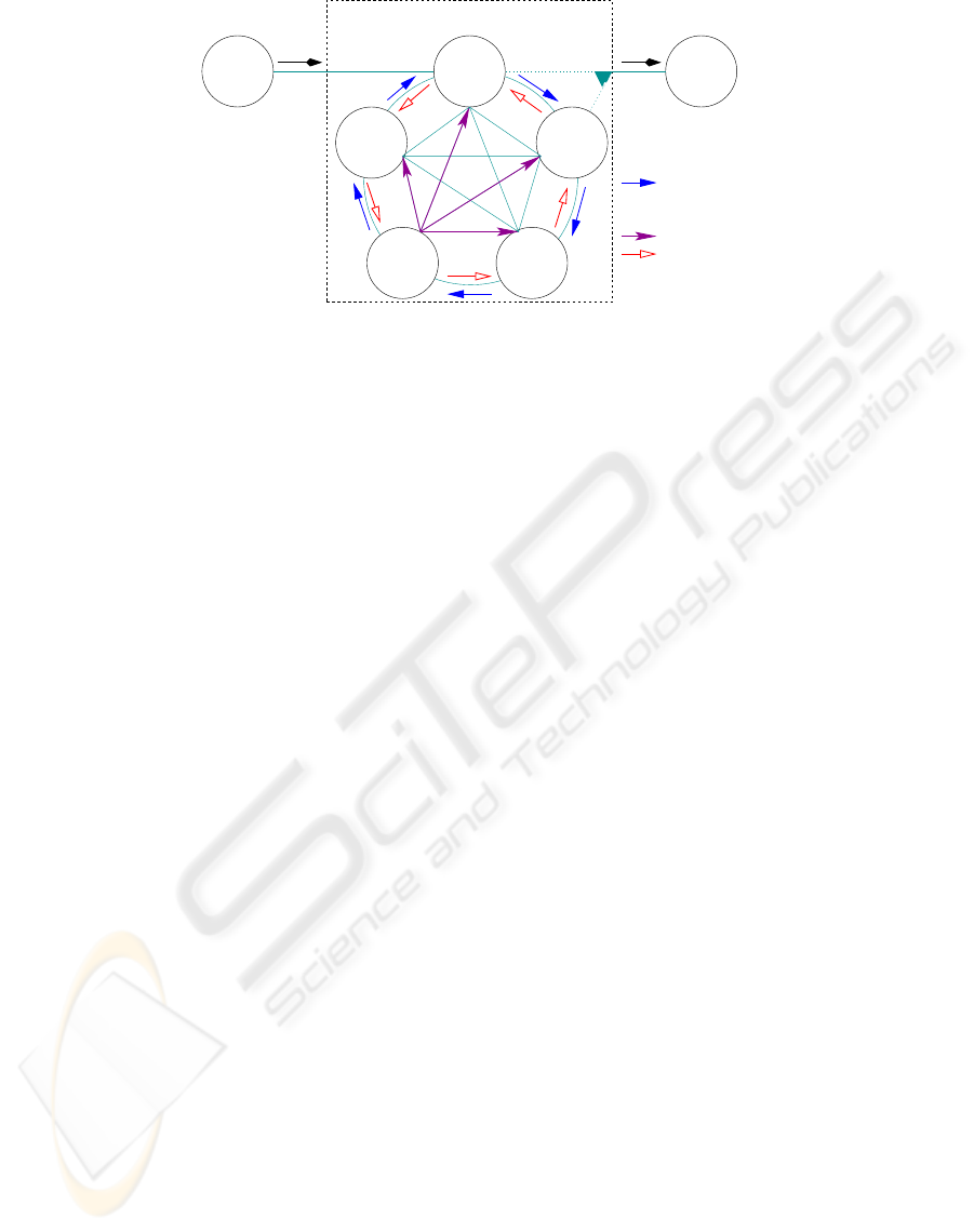
Figure 5 illustrates the design of the distributed

branch and bound (DBB) skeleton provided by the

Muesli skeleton library. It consists of a set of peer

solvers, which exchange problems, solutions, and

(possibly) load information. Several topologies for

connecting the solvers are possible. For small num-

bers of processors, a ring topology can be used, since

it enables an easy termination detection. For larger

numbers of processors, topologies like torus or hyper-

cube may lead to a faster propagation of work from

hot spots to idle processors. For simplicity, we will

assume a ring topology in the sequel. Compared to

more complicated topologies the ring also simpliﬁes

the dynamic adaption of the number of workers in

case that more or less computation capacity has to be

devoted to the branch & bound skeleton within the

overall computation. This (not yet implemented) fea-

ture will enable a well-balanced overall computation.

In our example, n = 5 solvers are used. Each

solver maintains its own local work pool and has one

entrance and one exit. Exactly one of the solvers,

called the master solver, serves as an entrance to the

DBB-skeleton and receives new optimization prob-

lems from the predecessor. Any of the n solvers may

deliver the detected optimal solution to the successor

of the branch & bound skeleton in the overall process

topology. All solvers know each other for a fast distri-

bution of newly detected best solutions

. If the skele-

ton only consists of a single solver neither communi-

cation nor distributed termination detection are nec-

essary. In this case all communication parts as well

as the distributed termination detection algorithm are

bypassed to speed up the computation.

The code fragment in Fig. 4 shows an example

application of our distributed B&B skeleton. It con-

structs the process topology depicted in Fig. 5. Work

request messages are only sent when using a demand-

driven work distribution.

The construction of the process topology resem-

bles that in the previous example. Instead of a ﬁlter a

BBSolver process is used as a worker. In addition to

the betterThan and isSolution function two

other argument functions are passed to the construc-

tor, namely a branch and a bound function. The

constructor DistributedBB produces n copies of

the solver. One of the solvers is automatically chosen

as the master solver.

As described in the previous section, a task-parallel

skeleton consumes a stream of input values and pro-

duces a stream of output values. If the master solver

receives a new optimization problem, the communica-

tion with the predecessor is blocked until the received

Thus, the topology is in fact a kind of wheel with

spokes rather than a ring.

int main(int argc, char

argv) {

InitSkeletons(argc,argv);

// step 1: create a process topology

Initial<Problem> initial(generateProblem);

BBSolver<Problem> solver("ring",branch,bound,

betterThan,isSolution);

DistributedBB<Problem> bnb =

DistributedBB<Problem>(solver,n);

Final<Problem> final(fin);

Pipe pipe(initial,bnb,final);

// step 2: start process topology

pipe.start();

TerminateSkeletons();

}

Figure 4: Task parallel example application of a fully dis-

tributed Branch and Bound skeleton.

problem is solved. This ensures that the skeleton pro-

cesses only one optimization problem at a time. There

are different variants for the initialization of paral-

lel branch & bound algorithms with the objective of

providing each worker with a certain amount of work

within the start-up phase. Ideally, the work load is

distributed equally to all workers. However, the work

load is hard to predict without any domain knowledge.

For this reason the skeleton uses the most common

approach, namely root initialization, i.e. the root of

the state space tree is inserted into the local work pool

of the master solver. Subproblems are distributed ac-

cording to the load balancing scheme applied by the

solvers. This initialization has the advantage that it is

very easy to implement and no additional code is nec-

essary. Other initialization strategies are discussed in

the literature. A good survey can be found in (Hen-

rich, 1994a).

Each worker repeatedly executes two phases: a

communication phase and a solution phase. Let us

ﬁrst consider the communication phase. In order to

avoid that computation time is wasted with the solu-

tion of irrelevant subproblems, it is essential to spread

and process new best solutions as quickly as possible.

For this reason, we distinguish problem messages and

incumbent messages. Each solver ﬁrst checks for ar-

riving incumbents with MPI Testsome. If it has re-

ceived new incumbents, the solver stores the best and

discards the others. Moreover, it removes subprob-

lems whose lower bound is worse than the incumbent

from the work pool. Then, it checks for arriving sub-

problems and stores them in the work pool, if their

lower bounds are better than the incumbent.

The solution phase starts with selecting an unex-

amined subproblem from the work pool. As in the

master/worker design, the work pool is organized as

a heap and the selection rule implements a best-ﬁrst

search strategy. The selected problem is decomposed

into m subproblems by applying branch. For each

ALGORITHMIC SKELETONS FOR BRANCH & BOUND

295

...

problems +

termination

detection

BBSolver

BBSolver BBSolver

BBSolver

Initial BBSolver Final

Predecessor

Master Solver

B&B with distributed work pool

Worker

Successor

work requests

incumbents

initial

problem

optimal

solution

Figure 5: Branch & bound skeleton with distributed work pool.

of the subproblems, we proceed as follows. First, we

check, whether it is solved. If a new best solution is

detected, we update the local incumbent and broad-

cast it. A worse solution is discarded. Finally, if the

subproblem is not yet solved, the bound function is

applied and the subproblem is stored in the work pool

(see Fig. 5).

3.3 Load Distribution and

Knowledge Sharing

Since the work pools of the different solvers, grow

and shrink differently, some load balancing mecha-

nism is required. Many global and local load dis-

tribution schemes have been studied in the literature

(Henrich, 1994b; Henrich, 1995; R. L

uling, 1992;

N. Mahapatra, 1998; Sanders, 1998; A. Shina, 1992)

and many of them are suited in the context of a dis-

tributed branch & bound skeleton. Here, we will fo-

cus on two local load balancing schemes, a supply-

and a demand-driven one. The local schemes avoid

the larger overhead of a global scheme. On the other

hand, they need more time to distribute work over

long distances.

With the simple supply-driven scheme, each

worker sends in each ith iteration its second best prob-

lem to its right neighbor in the ring topology. It al-

ways processes the best problem itself, in order to

avoid communication overhead compared to the se-

quential algorithm. The supply driven approach has

the advantage that it distributes work slightly more

quickly than a demand driven approach, since there

is no need for work requests. This may be beneﬁcial

in the beginning of the computation. A major dis-

advantage of this approach is that many subproblems

are transmitted in vain, since they will be sooner or

later discarded at their destination due to better in-

cumbents, in particular for small i. Thus, high com-

munication costs are caused.

The demand-driven approach distributes load only

in case that a neighbor requests it. In our case, a

neighbor sends the lower bound of the best problem

in its work pool (see Fig. 5). If this value is worse

than the lower bound of the second best problem of

the worker receiving this information, it is interpreted

as a work request and a problem is transmitted to the

neighbor. In case that the work pool of the neigh-

bor is empty, the information message indicates this

fact rather than transmitting a lower bound. An in-

formation message is sent every ith iteration of the

main loop. In order to avoid ﬂooding the network

with ”empty work pool” messages, such messages are

never sent twice. If the receiver of an “empty work

pool message” is idle, too, it stores this request and

serves it as soon as possible. The advantage of this

algorithm is that distributing load only occurs, if it

is necessary and beneﬁcial. The overhead of sending

load information messages is very low due to their

small sizes. For small i the overhead is bigger, but

idle processors get work more quickly.

3.4 Termination Detection

In the distributed setting, it is harder to detect that the

computation has ﬁnished and the optimal solution has

been found. The termination detection algorithm used

in the DBB-skeleton is a variant of Dijkstra’s algo-

rithm outlined in (Quinn, 1994). Our implementation

utilizes the speciﬁc property of MPI that the order in

which messages are received from a sender S is al-

ways equal to the order in which they were sent by S.

This characteristic can be used for the purpose of ter-

mination detection in connection with local load dis-

tribution strategies as described above.

As mentioned, we arrange the workers in a ring

topology, since this renders the termination detection

particularly easy and simpliﬁes the dynamic addition

and removal of workers. For a small number of pro-

cessors (as in our system), the large diameter of the

ICSOFT 2006 - INTERNATIONAL CONFERENCE ON SOFTWARE AND DATA TECHNOLOGIES

296

1234567891011121314

#workers

centralized workpool

distributed workpool, supply driven work

distribution

distributed workpool, demand driven work

distribution

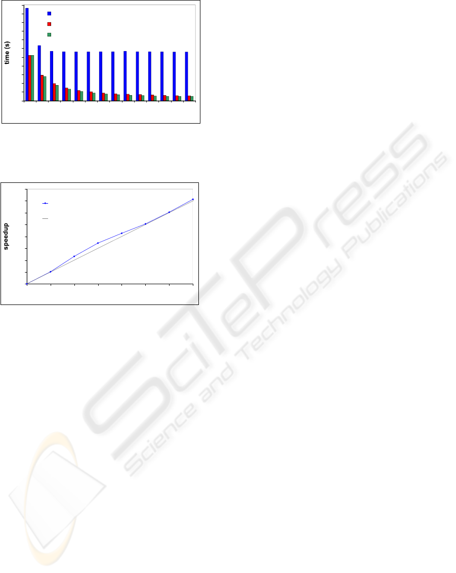
Figure 6: Runtimes for the 16 city TSP using the cen-

tral work pool manager and the distributed work pool with

supply- and demand-driven work distribution depending on

the number of workers.

1,00

2,00

3,00

4,00

5,00

6,00

7,00

8,00

9,00

12345678

#workers

distrributed workpool, demand

driven work distribution

linear speedup

Figure 7: Speedups for the 30 city TSP using the distributed

work pool with demand-driven work distribution depend-

ing on the number of workers. The speedups are the aver-

ages taken from 300 runs with different, randomly gener-

ated maps.

ring topology is no serious problem for the distribu-

tion of work.

Let n be the number of solvers of the DBB-

skeleton. When the master solver receives a new op-

timization problem, it initializes the termination de-

tection by sending a token along the ring in the same

direction as the load is distributed. The token only

consists of an int value. Initially, the token has the

value n. If a solver receives a new subproblem, this

event is noted by setting a ﬂag to true. On arrival of

a token the solver uses the rules stated by the follow-

ing pseudo code:

IF (workpool is empty AND flag == false)

token := token - 1;

IF (workpool is not empty OR flag == true) {

token := n; flag := false; }

IF (token > 0) send token to successor;

IF (token == 0) computation is finished;

Only if all workers are idle, the token is decremented

by every worker and the computation is ﬁnished. No

more problems can be in the network, since the token

cannot overtake other messages on its way. Note that

this algorithm only works for load balancing strate-

gies which send load in the same direction as the to-

ken.

4 EXPERIMENTAL RESULTS

We have tested the different versions of the branch &

bound skeleton experimentally on a IBM workstation

cluster (ZIV, 2006) using up to 16 Intel Xeon EM64T

processors with 3.6 GHz, 1 MB L2 Cache, and 4 GB

memory, connected by a Myrinet (Myricom, 2006).

As example applications we have considered the n-

puzzle as explained in section 2 as well as a parallel

version of the traveling salesman problem (TSP) al-

gorithm by Little et al. (J.D.C. Little, 1963). Both

differ w.r.t. the quality of their bounding functions

and hence in the number of considered irrelevant sub-

problems.

The presented B&B algorithm for the n-puzzle has

a rather bad bounding function based on the Manhat-

tan distance of each tile to its destination. It is bad,

since the computed lower bounds are often much be-

low the value of the best solution. As a consequence,

the best-ﬁrst search strategy is not very effective and

the number of problems considered by the parallel

skeleton differs enormously over several runs with the

same inputs. This number largely depends on the fact

whether a subproblem leading to the optimal solution

is picked up early or late. Note that the parallel al-

gorithm behaves non-deterministically in the way the

search-space tree is explored. In order to get reliable

results, we have repeated each run 100 times and com-

puted the average runtimes.

The goal of the TSP is to ﬁnd the shortest round trip

through n cities. Little’s algorithm represents each

problem by its residual adjacency matrix, a set of cho-

sen edges representing a partially completed tour, and

a lower bound on the length of any full tour, which

can be generated by extending the given partial tour.

New problems are produced by selecting a key edge

and generating two new problems, in which the cho-

sen edge is included and excluded from the emerging

tour, respectively. The key edge is selected based on

the impact that the exclusion of the edge will have

on the lower bound. The lower bounds are computed

based on the fact that each city has to be entered and

left once and that consequently one value in every row

and column of the adjacency matrix has to be picked.

The processing of a problem mainly requires three

passes through the adjacency matrix.

The TSP algorithm computes rather precise lower

bounds. Thus, the best-ﬁrst strategy works ﬁne, and

the parallel implementation based on Quinn’s formu-

lation of the algorithm (Quinn, 1994) considers only

very few problems more than the sequential algo-

rithm, as explained below.

ALGORITHMIC SKELETONS FOR BRANCH & BOUND

297

0,00

1,00

2,00

3,00

4,00

5,00

6,00

7,00

8,00

12345678

#workers

centralized workpool

distributed workpool, demand

driven work distribution

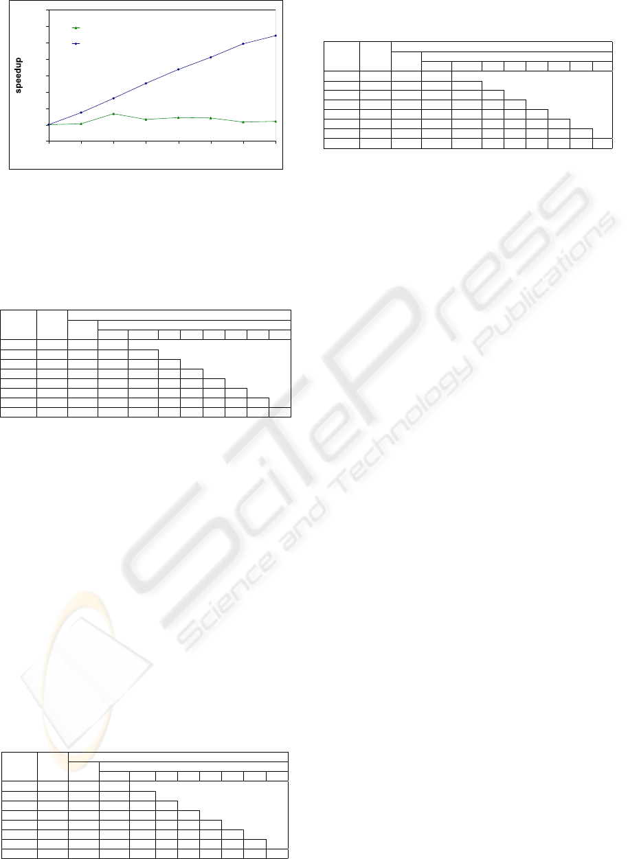
Figure 8: Speedups for 24-puzzle using the central work

pool manager and the distributed work pool with demand-

driven work distribution depending on the number of work-

ers.

Table 1: Distribution of problems for the 16 city TSP using

a distributed work pool and demand driven work distribu-

tion.

# considered problems

#workers runtime worker

(s) total 1 2 3 4 5 6 7 8

1 10.38 263019 263019

2 5.54 274002 139922 134080

3 3.52 263583 90783 86039 86761

4 2.64 262794 66536 65141 65475 65642

5 2.10 273175 55863 52386 55993 53878 55055

6 1.74 270525 45916 45150 44938 45574 42638 46309

7 1.52 263180 39495 38749 37492 37197 37134 36273 36840

8 1.35 265698 34196 33763 33525 32793 32424 32466 32231 34300

Consequently, the runtimes were relatively similar

over several runs with the same parameters. For the

TSP, we have used a real world 16 city map taken and

adapted from (Reinelt, 1991) and 300 randomly gen-

erated 30 city maps. The real world map has much

more sub-tours with similar lengths. Thus, propor-

tionally more subproblems are processed which do

not lead to the optimal solution than for the artiﬁcial

map, where the best solution is found more easily.

When comparing the supply- and the demand-

driven approach (see Figure 6 and the 3rd columns

of Tables 1, 2), we notice that, as expected, the de-

mand driven scheme is better, since it produces less

communication overhead. The fact that the problems

are distributed slightly slower causes no serious per-

Table 2: Distribution of problems for the 16 city TSP using

a distributed work pool and supply driven work distribution.

# considered problems

#workers runtime worker

(s) total 1 2 3 4 5 6 7 8

1 10.38 263019 263019

2 5.84 262522 162536 99986

3 3.92 271179 93060 89886 88233

4 2.91 269021 66004 67709 66572 68736

5 2.32 271717 53161 54569 55420 55074 53493

6 2.03 265100 43227 47420 47739 42342 42185 42187

7 1.75 265862 34390 34701 35100 36693 37917 51595 35466

8 1.35 264509 44379 32157 29789 29228 30017 31704 33124 34111

Table 3: Distribution of problems for the 16 city TSP using

a central work pool manager.

# considered problems

#workers runtime worker

(s) total 1 2 3 4 5 6 7 8

1 22.01 263018 263018

2 12.74 267057 133808 133249

3 11.41 267019 116339 104349 46331

4 11.26 267030 115396 103522 45945 2167

5 11.26 267039 116064 103735 45406 1712 106

6 11.25 267199 116082 103679 45470 1791 123 54

7 11.26 267050 114111 103167 46558 2767 319 89 39

8 11.25 267024 115671 103675 45227 2071 226 81 45 28

formance penalty.

For the supply driven scheme, we have used an

optimal number i for the amount of iterations that a

worker waits before delegating a problem to a neigh-

bor. If i is chosen too large, important problems will

not spread out fast enough. If i is too small, the com-

munication overhead will be too large. We found that

the optimal value for i depends on the application

problem and on the number of workers. If the number

of workers increases, i has to be increased as well. In

our experiments, the optimal values for i were ranging

between 2 and 20 for up to 8 workers.

As expected, we see that for the centralized B&B

skeleton the work pool manager quickly becomes a

bottleneck and it has difﬁculties to keep more than 2

workers busy (see Figures 6, 8 and Table 3). This

is due to the fact that the amount of computations

done for a problem is linear in the size of the prob-

lem, just as the communication complexity for send-

ing and receiving a problem. Thus, relatively little is

gained by delegating a problem to a worker. The work

pool manager has to spend only little work less for

transmitting the problem than its processing would re-

quire. This property is typical for virtually all practi-

cally relevant branch & bound problems we are aware

of. It has the important consequence that a centralized

work pool manager does not work well for branch &

bound on distributed memory machines. Also note

that the centralized scheme needs one more proces-

sor, the work pool manager, than the distributed one

rendering this approach even less attractive.

Both variants of the design with a distributed work

pool do not have these drawbacks (see Figures 6, 7,

8 and Tables 1, 2). Here, the communication over-

head is much smaller. Each worker fetches most prob-

lems from its own work pool, such that they require

no communication. This is particularly true for the

demand driven approach. This scheme has the advan-

tage that after some start-up phase, in which all work-

ers are supplied with problems, there is relatively little

communication and the workers mainly process lo-

cally available problems. This is essential for achiev-

ing good runtimes and speedups. We anticipate that

this insight not only applies to branch & bound but

also to other skeletons with a similar characteristic

ICSOFT 2006 - INTERNATIONAL CONFERENCE ON SOFTWARE AND DATA TECHNOLOGIES

298

such as divide & conquer and other search skeletons.

We are currently working on experimental results sup-

porting this claim.

Interestingly we could even observe slightly super-

linear speedups for the 30 city TSPs. They can be

explained by the fact that a parallel B&B algorithm

may tackle important subproblems earlier than the se-

quential one, since it processes the state-space tree in

a different order (T. Lai, 1984).

It is clear that a parallel B&B algorithm will typ-

ically consider more problems than a correspond-

ing sequential one, since it eagerly processes several

problems in parallel, which would be discarded in the

sequential case, since their lower bounds are worse

than a detected solution. Interestingly for both con-

sidered example applications, TSP and n-puzzle, the

corresponding overhead was very small and only few

additional problems have been processed by the par-

allel implementation (see the 3rd columns of Tables

1, 2, 3). For instance, for the 16 city TSP no more

than 274002 − 263019 = 10983 additional problems

are processed by the parallel algorithm; this is less

than 4.2 %. This is essential for achieving reasonable

speedups.

As an implementation detail of the centralized ap-

proach let us mention that it is important that the work

pool manager receives in each iteration all available

subproblems and solutions from the workers rather

than just one of them. The reason is that MPI Waitany

(used internally) is unfair and that an overloaded work

pool manager will hence almost exclusively commu-

nicate with a small number of workers. If a starving

worker has an important subproblem (one that leads

to the optimal solution) or a good solution, which it is

not able to deliver to the work pool manager, this will

cause very bad runtimes.

Another implementation detail of the centralized

approach concerns the amount of buffering. In order

to be able to overlap computation and communica-

tion, it is a good idea that the work pool manager not

only sends one problem to each worker and then waits

for the results, but that it sends m problems such that

the worker can directly tackle the next problem af-

ter ﬁnishing the previous one. Here it turned out that

one has to be careful not to choose m too large, since

then problems which would otherwise be discarded

due to appearing better incumbents will be processed

(in vain). In our experiments, m = 2 was a good

choice.

5 CONCLUSION

We have considered two different implementation

schemes for the branch & bound skeleton. Besides

a simple approach with a central work pool manager,

we have investigated a scheme with a distributed work

pool. As our analysis and experimental results show,

the communication overhead is high for the central-

ized approach and the work pool manager quickly be-

comes a bottleneck, in particular, if the number of

computation steps for each problem grows linearly

with the problem size, as it is the case for virtually all

practically relevant branch & bound problems. Thus,

the centralized scheme does not work well in practice.

On the other hand, our scheme with a distributed

work pool works ﬁne and provides good runtimes and

scalability. The latter is not trivial, as discussed e.g. in

the book of Quinn (Quinn, 1994), since parallel B&B

algorithms tend to process an increasing number of ir-

relevant problems the more processors are employed.

In particular, the demand-driven design works well

due to its low communication overhead.

For the supply-driven approach, we have investi-

gated, how often a problem should be propagated to a

neighbor. Depending on the application and the num-

ber of workers, we have observed the best runtimes, if

a problem was delegated between every 2nd and every

20th iteration.

We are not aware of any previous comparison of

different implementation schemes of branch & bound

skeletons for MIMD machines with distributed mem-

ory in the literature. In the MaLLBa project (E. Alba,

2002; F. Almeida, 2001), a branch & bound skeleton

based on a master/worker approach and a queue for

storing subproblems has been developed. But as we

pointed out above, this scheme is more suitable for

shared memory machines than for distributed mem-

ory machines. Hofstedt (Hofstedt, 1998) sketches a

B&B skeleton with a distributed work pool. Here,

work is only delegated, if a local work pool is empty.

A quick propagation of “interesting” subproblems are

missing. According to our experience, this leads to a

suboptimal behavior. Moreover, Hofstedt gives only

few experimental results based on reduction steps in

a functional programming setting rather than actual

runtimes and speedups.

As future work, we intend to investigate alternative

implementation schemes of skeletons for other search

algorithms and for divide & conquer.

REFERENCES

A. Benoit, M. Cole, J. H. S. G. (2005). Flexible skeletal pro-

gramming with eskel. In Proc. EuroPar 2005. LNCS

3648, 761–770, Springer Verlag, 2005.

A. Shina, L. K. (1992). A load balancing strategy for

prioritized execution of tasks. In Proc. Workshop

on Dynamic Object Placement and Load Balancing,

ECOOP’92.

Cole, M. (1989). Algorithmic Skeletons: Structured Man-

agement of Parallel Computation. MIT Press.

ALGORITHMIC SKELETONS FOR BRANCH & BOUND

299

Cole, M. (2004). Bringing skeletons out of the closet:

A pragmatic manifesto for skeletal parallel program-

ming. In Parallel Computing 30(3), 389–406.

Cole, M. (2006). The skeletal parallelism web page.

http://homepages.inf.ed.ac.uk/mic/Skeletons/.

E. Alba, F. Almeida, e. a. (2002). Mallba: A library of

skeletons for combinatorial search. In Proc. Euro-Par

2002. LNCS 2400, 927–932, Springer Verlag, 2005.

F. Almeida, I. Dorta, e. a. (2001). Mallba: Branch and

bound paradigm. In Technical Report DT-01-2. Uni-

versity of La Laguna, Spain, Dpto. Estadistica , I.O. y

Computacion.

G. H. Botorog, H. K. (1996). Efﬁcient parallel program-

ming with algorithmic skeletons. In Proc. Euro-

Par’96. LNCS 1123, 718–731, Springer Verlag, 1996.

G. H. Botorog, H. K. (1998). Efﬁcient high-level parallel

programming. In Theoretical Computer Science 196,

71–107.

G.L. Nemhauser, L. W. (1999). Integer and combinatorial

optimization. Wiley.

H. Kuchen, R. Plasmeijer, H. S. (1994). Efﬁcient distributed

memory implementation of a data parallel functional

language. In Proc. PARLE’94. LNCS 817, 466–475,

Springer Verlag.

H. Kuchen, M. C. (2002). The integration of task and

data parallel skeletons. In Parallel Processing Letters

12(2), 141–155.

Henrich, D. (1994a). Initialization of parallel branch-and-

bound algorithms. In Proc. 2nd International Work-

shop on Parallel Processing for Artiﬁcial Intelligence

(PPAI-93). Elsevier.

Henrich, D. (1994b). Local load balancing for data-parallel

branch-and-bound. In Proc. Massively Parallel Pro-

cessing Applications and Development, 227-234.

Henrich, D. (1995). Lastverteilung fuer feinkoernig par-

allelisiertes branch-and-bound. In PhD Thesis. TH

Karlsruhe.

Hofstedt, P. (1998). Task parallel skeletons for irregu-

larly structured problems. In Proc. EuroPar’98. LNCS

1470, 676 – 681, Springer Verlag.

I. Dorta, C. Leon, C. R. A. R. (2003). Parallel skeletons for

divide and conquer and branch and bound techniques.

In Proc. 11th Euromicro Conference on Parallel, Dis-

tributed and Network-based Processing (PDP2003).

J. Clausen, M. P. (1999). On the best search strategy in par-

allel branch-and-bound: Best-ﬁrst search versus lazy

depth-ﬁrst search search. In Annals of Operations Re-

search 90, 1-17 .

J.D.C. Little, K.G. Murty, D. S. C. K. (1963). An algorithm

for the traveling salesman problem. In Operations Re-

search 11, 972–989 .

Kuchen, H. (2002). A skeleton library. In Euro-Par’02.

LNCS 2400, 620–629, Springer Verlag.

Kuchen, H. (2004). Optimizing sequences of skeleton

calls. In Domain-Speciﬁc Program Generation. LNCS

3016, 254–273, Springer Verlag.

Kuchen, H. (2006). The skeleton li-

brary web pages. http://www.wi.uni-

muenster.de/PI/forschung/Skeletons/index.php.

MPI (2006). Message passing interface forum, mpi.

In MPI: A Message-Passing Interface Standard.

http://www.mpi-forum.org/docs/mpi-11-html/mpi-

report.html.

Myricom (2006). The myricom homepage.

http://www.myri.com/.

N. Mahapatra, S. D. (1998). Adaptive quality equaliz-

ing: High-performance load balancing for parallel

branch-and-bound across applications and computing

systems. In Proc. International Parallel Processing

and Distributed Processing Symposium (IPDPS98).

Pelagatti, S. (2003). Task and data parallelism in p3l. In

Patterns and Skeletons for Parallel and Distributed

Computing. eds. F.A. Rabhi, S. Gorlatch, 155–186,

Springer Verlag.

Quinn, M. (1994). Parallel Computing: Theory and Prac-

tice. McGraw Hill.

R. Bisseling, I. F. (2005). Mondriaan sparse matrix parti-

tioning for attacking cryptosystems – a case study. In

to appear in Proceedings of ParCo 2005, Malaga.

R. L

uling, B. M. (1992). Load balancing for distributed

branch and bound algorithms. In Proc. 6th Interna-

tional Parallel Processing Symposium (IPPS92), 543-

549. IEEE.

Reinelt, G. (1991). Tsplib – a traveling salesman

problem library. In ORSA Journal on Comput-

ing 3, 376–384. see also: http://www.iwr.uni-

heidelberg.de/groups/comopt/software/TSPLIB95/

(gr17).

Sanders, P. (1998). Tree shaped computations as a model

for parallel applications. In Proc. Workshop on Appli-

cation Based Load Balancing (ALV’98). TU Munich.

T. Lai, S. S. (1984). Anomalies in parallel branch-and-

bound algorithms. In Communications of the ACM

27, 594–602.

Trienekens, H. (1990). Parallel branch & bound algorithms.

In PhD Thesis. University of Rotterdam.

W. Gropp, E. Lusk, A. S. (1999). Using MPI. MIT Press.

Y. Shinano, M. Higaki, R. H. (1995). A generalized util-

ity for parallel branch and bound algorithms. In Proc.

7th IEEE Symposium on Parallel and Distributed Pro-

cessing, 392–401. IEEE.

Y. Shinano, M. Higaki, R. H. (1997). Control schemes in a

generalized utility for parallel branch and bound algo-

rithms. In Proc. 11th International Parallel Process-

ing Symposium, 621–627. IEEE.

Y. Xu, T. Ralphs, L. L. M. S. (2005). Alps: A framework

for implementing parallel tree search algorithms. In

Proc. 9th INFORMS Computing Society Conference.

ZIV (2006). Ziv-cluster. http://zivcluster.uni-muenster.de/.

ICSOFT 2006 - INTERNATIONAL CONFERENCE ON SOFTWARE AND DATA TECHNOLOGIES

300