
APPROXIMATE REASONING TO LEARN
CLASSIFICATION RULES
Amel Borgi
Research Unit SOIE, ISG, Tunis
National Institute of Applied Science and Technology, INSAT
Centre Urbain Nord de Tunis, BP 676, 1080 Tunis, Tunisia
Keywords: Supervised learning, rules generation, approximate reasoning, infere
nce engine, imprecision and uncertainty
management.
Abstract: In this paper, we propose an original use of approximate reasoning not only
as a mode of inference but also
as a means to refine a learning process. This work is done within the framework of the supervised learning
method SUCRAGE which is based on automatic generation of classification rules. Production rules whose
conclusions are accompanied by belief degrees, are obtained by supervised learning from a training set.
These rules are then exploited by a basic inference engine: it fires only the rules with which the new
observation to classify matches exactly. To introduce more flexibility, this engine was extended to an
approximate inference which allows to fire rules not too far from the new observation. In this paper, we
propose to use approximate reasoning to generate new rules with widened premises: thus imprecision of the
observations are taken into account and problems due to the discretization of continuous attributes are
eased. The objective is then to exploit the new base of rules by a basic inference engine, easier to interpret.
The proposed method was implemented and experimental tests were carried out.
1 INTRODUCTION
Facing the increase of data amount recorded daily,
the detection of both structures and specific links
between them, the organisation and the search of
exploitable knowledge have become a strategic
stake for decision making and prediction task. This
complex problem of data mining has multiple
aspects (Michalski et al., 1983) (Zhou, 2003). We
focus on one of them: supervised learning. In
(Borgi, 1999) (Borgi et al. 2001), we have proposed
a learning method from examples situated at the
junction of statistical methods and those based on
Artificial Intelligence techniques. Our method,
SUCRAGE (SUpervised Classification by Rules
Automatic GEneration) is based on automatic
generation of classification rules. Production rules
IF premise THEN conclusion are a mode of
knowledge representation widely used in learning
systems because they ensure the transparency and
the easy explanation of the classifier (Duch et al.,
2004) (Haton et al., 1991). Indeed, the construction
of production rules using the knowledge and the
know-how of an expert is a very difficult task. The
complexity and cost of such a knowledge acquisition
have led to an important development of learning
methods used for an automatic knowledge
extraction, and in particular for rules extraction
(Haton et al. 1991) (Duch et al., 2004).
The learning method SUCRAGE is based on a
correl
ation search among the features of the
examples and on discretization of continuous
attributes. Rules conclusions are of the form
«belonging to a class » and are uncertain. In the
classification phase, an inference engine exploits the
base of rules to classify new observations and also
manages rules uncertainty. This reasoning that we
called basic reasoning allows to obtain conclusions,
when the observed facts match exactly rules
premises.
In this paper, we are interested in an other
reasoni
ng: approximate reasoning (Zadeh, 1979)
(Haton et al. 1991) (El-Sayed, et al., 2003). It allows
to introduce more flexibility and to overcome
problems due to discretization. Such reasoning is
closer to human reasoning than the basic one:
203
Borgi A. (2006).
APPROXIMATE REASONING TO LEARN CLASSIFICATION RULES.
In Proceedings of the First International Conference on Software and Data Technologies, pages 203-210
DOI: 10.5220/0001310402030210
Copyright
c
SciTePress
human inferences do not always require a perfect
correspondence between facts or causes to conclude.
In (Borgi et al., 2001), we have proposed a
context-oriented approximate reasoning. This
reasoning, used as an inference mode, allows to
manage imprecise knowledge as well as rules
uncertainty: according to distance between
observations and premises, it computes a
neighborhood degree and associates a final
confidence degree to rules conclusions. This model
is faithful to the classical scheme of Generalized
Modus Ponens (Zadeh, 1979). In this paper, we
propose to see approximate reasoning under another
angle. The originality of our approach lies in the use
of approximate reasoning, not only as a mode of
inference, but to refine the learning. This reasoning
allows to generate new rules and to ease in this way
problems due to discretization and imprecision of
the observations. The aim is that the new base of
rules will then be exploited by a basic inference
engine more easy to interpret. In our model,
approximate reasoning has then no more vocation to
be a method of inference allowing to fire certain
rules but joins in the process of learning itself. The
software SUCRAGE was extended: new rules
construction through approximate reasoning was
implemented. Applications of the extended version
to benchmark problems are reported.
This paper is organized as follows. In section 2,
the method SUCRAGE is described. More precisely
we describe the learning phase (rules generation)
and the classification phase. Only the basic
inference engine is presented. In section 3, we
present the approximate reasoning used as an
inference mode. Section 4 attempts to explain the
use of approximate reasoning to generate new
classification rules and its contribution to the
process of learning. Tests and results obtained by
computer simulations with two benchmarks are
provided in section 5. Finally, section 6 concludes
the study.
2 THE SUPERVISED LEARNING
METHOD SUCRAGE
2.1 Rules Generation
In this section, we describe the learning phase of the
supervised learning method SUCRAGE. The
training set contains examples described by
numerical features denoted X
1
, ..., X
i
, ..., X
p
. These
examples are labelled by the class to which they
belong. The classes ar
e denoted y ,y ,...,y
1 2 C
. The
generated rules are of the type:
A
1
and A
2
and ... and A
k
⎯⎯→ y, α
where
A
i
: condition of the form X
j
is in [a,b],
X
j
: the j
th
vector component representing an
observation,
[a,b]: interval issued from the discretization of
the features variation domain (here, it is the
variation domain of the feature X
j
),
y: a hypothesis about membership in a class,
α: a belief degree representing the uncertainty of
the conclusion.
rg_0 rg_1 rg_2 rg_3
X
4
X
5
rg_0 rg_1 rg_2 rg_3
premise :
X
4
is in rg_3 and X
5
is in rg_2
rg_0 rg_1 rg_2 rg_3
X
4
X
5
rg_0 rg_1 rg_2 rg_3
premise :
X
4
is in rg_3 and X
5
is in rg_2
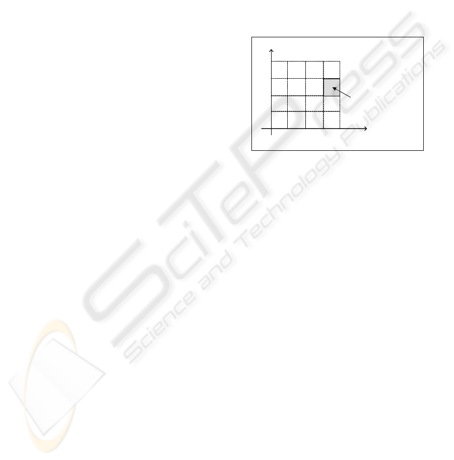
Figure 1: A partition of the correlated features space.
Our approach is multi-featured as the features
that appear in rules premises are selected in one
piece. This selection is realized by linear correlation
search among the training set elements (Borgi,
1999) (Borgi et al., 2001). So the first step consists
in computing the correlation matrix between the
components of the training set vectors. Then to
decide which components are correlated, this matrix
is thresholded (with a threshold denoted θ). The idea
is to detect privileged correlations between the
features and to generate the rules according to these
correlations. According to Vernazza’s approach, we
decide to group in the same premises all components
that are correlated (Vernazza, 1993).
Next step in building the rules is feature
discretization. Among the non supervised methods
of discretization, the simplest one leads to M sub-
ranges of equal width. This method called the
regular discretization is the one we retain for this
study. The M obtained sub-ranges are denoted rg_0,
rg_1, ..., rg_(M-1), these values are totally ordered.
Once the discretization done, condition parts of
rules are then obtained by considering for each
correlated components subset, a sub-interval (rg_i)
for each component in all possible combinations.
Indeed the premises of the rules form a partition of
the correlated components space. Figure 1 illustrates
such a partition in the case of two correlated features
(X
4
and X
5
) and with a subdivision size M=4.
ICSOFT 2006 - INTERNATIONAL CONFERENCE ON SOFTWARE AND DATA TECHNOLOGIES
204

Each premise that we construct leads to the
generation of C rules (C: number of classes). The
rules conclusions are of the form « belonging to a
class » and are not absolutely certain, that’s why
each conclusion is accompanied by a belief degree
α
. In this paper, we propose to represent the belief
degrees by a classical probability estimated on the
training set (Pearl 90) (Borgi et al. 01) (Borgi, 99).
2.2 Basic Inference Engine
The rules were generated for the purpose of a further
classification use. In classification phase, the base of
rules is exploited to classify new objects that don’t
belong to the training set. To achieve this goal, our
approach consists in using a 0+ order inference
engine. The inputs of this engine are the base of
rules previously built and a vector representing the
object to classify. The inference engine associates
then a class to this vector.
We propose two reasoning models. The first one,
called basic reasoning is presented in this section.
The second one, the approximate reasoning, will be
detailed in section 3. The basic reasoning allows the
inference engine to fire only the rules with which
the new observation components match exactly. The
engine classifies each new observation using the
classical deduction reasoning. It has to manage the
rules’ uncertainty and take it into account within the
inference dynamic. Uncertainty management is done
by computations on the belief degrees of the fired
rules. Once the rules fired, we have to compute a
final belief degree associated with each class. For
this we propose to use a triangular co-norm (Gupta
et al., 91): the final belief degree associated to each
class is the result of this co-norm applied on the
probabilities of the fired rules that conclude to this
considered class. Experimental tests presented in
this paper were realized with the Zadeh co-norm
(max). Finally the winner class associated with the
new observation is the class for which the final
belief degree is maximum.
3 APPROXIMATE REASONING
Approximate reasoning, in a general way, makes
reference to any reasoning which treats imperfect
knowledge. This imperfection has multiple facets:
for instance the knowledge can be vague, imprecise,
or uncertain. In spite of such imperfections,
approximate reasoning allows to treat this
knowledge and to end in conclusions. In (Haton et
al. 1991), approximate reasoning concerns as well
the imprecision and uncertainty representation as
their treatment and propagation in a knowledge
based system. The term approximate reasoning has
however a particular meaning of a word introduced
by Zadeh in the field of Fuzzy Logic (Zadeh 1979)
(Yager, 2000). In this frame, approximate reasoning
corresponds to Generalized Modus Ponens who is
an extension of Modus Ponens in fuzzy data. This
definition of approximate reasoning is not
contradictory to the first one which is more general
and concerns all the forms of imperfections.
The approximate reasoning which we introduce
is situated in the intersection of these two
approaches. We are however more close to
"fuzziers” as far as we remain faithful to the
Generalized Modus Ponens (Zadeh 1979), but we
adapt it to a symbolic frame (Borgi 1999) (Borgi et
al. 01) (El-Sayed et al., 2003). We propose a model
of Approximate Reasoning which allows to
associate a final degree of confidence to the
conclusions (classes) on the basis of an imprecise
correspondance between rules and observations.
This reasoning does not fire only the rules the
premises of which are exactly verified by the new
observation, but also those who are not too much
taken away from this observation. Thus, we are in
the situation described in figure 2.
A
1
and A
2
and ... and A
n
B with a belief degree α
A’
1
is nearly A
1
A’
2
is nearly A
2
.
.
.
A’
n
is nearly A
n
B with a belief degree α’
uncertainty
imprecision
uncertainty
A
1
and A
2
and ... and A
n
B with a belief degree α
A’
1
is nearly A
1
A’
2
is nearly A
2
.
.
.
A’
n
is nearly A
n
B with a belief degree α’
uncertainty
imprecision
uncertainty
Figure 2: Particular case of Generalized Modus Ponens.
The consideration of observations close to rules
premises allows to overflow around these premises.
More exactly, it allows to extend beyond around the
intervals stemming from the discretization and to
ease so the problems of borders due to any
discretization. So that our approximate reasoning
can become operational, it is necessary to formalize
first of all the notion of neighborhood. Then, it is
necessary to model the approximate inference, that
is to determine the degree of the final conclusion
(α’) of the diagram shown on figure 2.
APPROXIMATE REASONING TO LEARN CLASSIFICATION RULES
205

3.1 Proximity between Observation
and Premise
In works about approximate reasoning, Zadeh
(Zadeh, 1979) stresses the necessary introduction of
a distance in order to define neighbouring facts. In
(Ruspini, 1991), a similarity degree between two
objects is introduced. In our case, to define the
notion of neighbourhood we have defined two types
of measure or distance (Borgi, 1999) (Borgi et al.,
2001). A distance that we call local distance will
measure the proximity of an observation element to
a premise element. These distances will then be
aggregated to obtain a global distance between the
observation and the whole premise.
3.1.1 A Local Distance
We consider, by concern of clearness, the following
rule:
X
1
in rg_r1 and X
2
in rg_r2 and... X
n
in rg_rn →
y
t
,α
which groups together in its premise the attributes
X
1
, X
2
, ...,X
n
. This rule does not lose in generality: it
can be obtained by renaming the attributes.
We note V=(v
1
,v
2
,...,v
n
) the elements of the
observation concerned by the premise. To compare
V with the following premise: X
1
is in rg_r1 and X
2
is in rg_r2 and ... and X
n
is in rg_rn, we begin by
making local comparisons between v
1
and X
1
is in
rg_r1, between v
2
and X
2
is in rg_r2 ... So we have
to define the local distances d
1
, d
2
, ..., d
n
of the
following schema:
A
1
and A
2
and ... and A
n
→B with a belief degree α
A’
1
d
1
-distant of A
1
A’
2
d
2
-distant of A
2
...
A’
n
d
n
-distant of A
n
⎯⎯⎯⎯⎯⎯⎯⎯⎯⎯⎯⎯⎯⎯⎯⎯⎯⎯⎯⎯⎯
B with a belief degree α’
More precisely it comes to determine the
following distances d
i
: v
1
is d
1
-distant from rg_r1,
…, v
n
is d
n
-distant from rg_rn where the distance is
the formal translation of the neighboring concept.
Rule premise (A
i
) associates discrete values (rg_0,
rg_1, ...,rg_(M-1)) to observation components. But
observations (A’
i
or v
i
) have numerical values. In
order to compare them, we introduce a numerical-
symbolic interface (Borgi 99). We split each interval
rg_k into M sub-intervals of equal range, denoted
σ
0
, σ
1
, .... We thus have a finer discretization, and
we obtain M*M sub-intervals (σ
0
, σ
1
..., σ
M*M-1
.).
Figure 3 illustrates such sub-intervals obtained with
M=3.
We can associate to each numerical value v
i
the
sub-interval σ
t
to which it belongs. The distance d
i
between v
i
and rg_ri is then defined as the number
of sub-intervals of type σ separating σ
t
from rg_ri.
Of course, d
i
is 0 if v
i
is in rg_ri. Thus, we obtain the
distance vector D=(d
1
,d
2
,…,d
n
) associated to every
pair (observation, premise) or (observation, rule).
3.1.2 A Global Distance
In order to make approximate inferences, we want to
aggregate the different local distances d
i
. The result
of this aggregation is a global distance that we note
g-distance, and on which we wish to confer some
properties (Borgi, 1999). One property that we
impose to that distance is to be very sensitive to little
variations of neighboring facts. This global distance
that measures distance between approximately equal
vectors can be insensitive when facts are very far
from each other. This g-distance has to either
measure the proximity between two nearby facts, or
indicate by a maximal value, that they are not
nearby. This is a proximity measure, and not a real
distance. This distance is represented by an integer
in [0, M-1]. In order to take into account the value
dispersion, we do not use tools like min-max
functions but we propose an aggregation based on a
“dispersion” function S
D
:
S
D
: [0..M-1] ⎯⎯→ IN
k ⎯⎯→ S
D
(k) =
∑
=
−
n
i
k
d
1
2
)
i
(
S
D
(k) allows, in a way similar to the variance, to
measure the dispersal of the local distances d
i
around k. We have then defined a global distance g-
dist as follows:
g-dist: [0..M×(M-1)]
n
⎯⎯→ [0..M-1]
(d
1
,d
2
, ...,d
n
) ⎯⎯→
))]k(
min
(max[
1
0
1
S
S
D
M
k
D
−
=
−
The global distance is presented with more
details in (Borgi 1999) and (Borgi et al. 2001). We
have notably proved that the proposed aggregated
distance satisfies the above mentioned property.
We can notice that it is possible to have g-
distance equal to 0, even if the distance vector is not
null. In other words, it is possible to have a global
distance equal to 0 for an observation that does not
satisfy the considered rule.
ICSOFT 2006 - INTERNATIONAL CONFERENCE ON SOFTWARE AND DATA TECHNOLOGIES
206

3.2 Approximate Inference
The use of approximate inference supposes that a
meta-knowledge exists in the system and allows it to
run. In our case the meta-knowledge gives the
possibility to bind imprecision (observation and
premise of rule) to uncertainty (conclusion degree).
This meta-knowledge has two complementary
aspects: the first hypothesis says that a weak
difference between observation and premise induces
that the conclusion part is not significantly modified.
For every rule, a stability area exists around the
premise of the rule. The second and stronger
hypothesis says that if the distance between
observation and premise increases, then uncertainty
of the conclusion increases too. A maximal distance
must give a maximal uncertainty (in our case, it
corresponds to the minimal belief degree, i.e. a
probability equal to zero) (Borgi, 1999).
The conclusion degree is weakened in
accordance with the global distance. In our model,
belief degrees (α) associated with rules are
numerical, so it is hoped to conserve a numerical
final degree (α’) for the whole coherence. To
compute the final belief degree α’of a conclusion
via the approximate reasoning, given the global
distance d (symbolic) between the premises and the
observation and α the belief degree (numerical) of
the conclusion of the fired rule, we propose the
following function F :
F : [0,1] × [0..M-1] ⎯⎯→ [0,1]
(α,d) ⎯⎯→
)
1
1.(
−
−
M
d
α
This formula includes the two aspects of the
meta-knowledge hypothesis mentioned above. It is
easy to observe that little imprecisions (in cases
where d=0) do not modify uncertainty. On the other
hand, a maximal distance (d=M-1) induces a
complete uncertainty (α’=0). We note that we find
back the basic reasoning in the limit case d=0.
4 APPROXIMATE REASONING
TO LEARN NEW RULES
In this part, we present the use of approximate
reasoning not as a mode of inference to exploit rules
in classification phase, but as a means to refine the
learning. The use of approximate reasoning during
the learning phase consists in generating new rules
the premises of which are widened. The method
consists in generating rules by using the basic
approach described in section 2 then to look
"around" the rules to verify if we cannot improve
them or add better rules. The objective is then to
exploit this base of rules thanks to a basic inference
engine by hoping to obtain results close to a basic
generation of rules exploited by an approximate
engine.
For reasons of legibility and simplicity, we shall
call the rules generation realized by SUCRAGE in
its initial version the basic generation. The
generation of rules completed by the construction of
new rules via approximate reasoning will be called
approximate generation.
4.1 Method with a Constant
Number of Rules
This approach can be summarized by: "from an
observation situated near the rules which we
generated with the basic method of SUCRAGE, we
verify if we cannot widen every rule to a rule of
better quality". This is made always by using the
same whole learning set.
To consider that an observation O is near a rule
R, we have to define a g-threshold, it is the maximal
value authorized by g-distance(O, R).
For every observation O near a rule R (the
mother rule) and having the same conclusion (class)
as the rule R, we are going to build a new rule (the
daughter rule R
daughter
):
- the premise of R
daughter
is that containing
Premise(R) and O the most restrictive possible and
convex by using the ranges (rg_ri) and the sub-
intervals of type σ,
- the class of the conclusion do not change,
- the belief degree of R
daughter
is recomputed on
the whole training set according to the new premise.
This new assessment of the belief degree of the
daughter rule built through approximate reasoning
allows integrating this reasoning into the learning
process.
The sentence "Premise containing Premise(R)
and O the most restrictive possible and convex by
using the ranges (rg_ri) and the sub-intervals of type
σ" means that to create the new premise, we start
from the ancient premise and we add to all the
conditions that O does not verify the intervals of
type σ which would allow O to verify it. R
daughter
contains in its premise the same attributes as the
mother rule R but with wider values. For instance, as
shown in figure 3, in the case of a discretization
with M=3, if the given value O
i
∈σ
4
and the
condition is X
i
is in rg_0 then the new condition will
be X
i
is in rg_0 ∪
σ
3
∪
σ
4
(by supposing naturally
APPROXIMATE REASONING TO LEARN CLASSIFICATION RULES
207

that the condition of threshold on the global distance
is verified).
Figure 3: An example of construction of a new rule
condition.
In the construction procedure of a new rule
which we presented, a couple (observation, rule)
verifying certain properties gives birth to a new rule.
Among the mother rule and all the daughter rules we
can generate, only the one who has the strongest
belief degree is kept. Thus the initial number of
rules does not change.
4.2 Method with Addition of Rules
We try here to widen the method of generation of a
new base of rules so that the best rule is not the only
one kept in the base. For that purpose, we use the
"raw force" and we add in the base of rules all the
rules that we can generate from each: a rule can then
lead to several new rules and either as previously to
a unique rule (that of stronger degree). This method
allows to create a wide base close to data but this
base, because of its size, becomes illegible as for
interpretation by an expert. It becomes then
necessary to optimize the size of the base of rules
(Duch et al., 2004) (Nozaki et al. 1994).
5 TESTS AND RESULTS
The system SUCRAGE that we initially developed
allows the generation of rules by the method
presented in section 2.1 as well as their exploitation
by an inference engine. This engine uses a basic
reasoning or approximate one (Borgi, 1999) (Borgi
et al., 2001).
We completed this system by a module
of rules generation via the approximate reasoning.
We tested this new application on two learning
bases stemming from the server of Irvine's
University: t
hose bases are Iris data and Wine data.
To compare the different results, we used the
same test methods with the same parameters values
for the classification system (size of subdivision M,
correlation threshold θ). We used a ten order cross-
validation (Kohavi, 1995). The obtained results are
presented and analyzed in this part.
5.1 Results of the Method with a
Constant Number of Rules
σ
0
σ
1
σ
2
σ
3
σ
4
σ
5
σ
6
σ
7
σ
8
rg_0 rg_1 rg_2
New condition
×
σ
0
σ
1
σ
2
σ
3
σ
4
σ
5
σ
6
σ
7
σ
8
rg_0 rg_1 rg_2
New condition
σ
0
σ
1
σ
2
σ
3
σ
4
σ
5
σ
6
σ
7
σ
8
rg_0 rg_1 rg_2
New condition
×
We present here the tests realized with the method
of new rules construction via the approximate
reasoning according to the approach with a constant
number of rules. The first tests were made with g-
threshold=0 or g-threshold=1 which seem the only
reasonable values. Values superior to 2 would throw
a search which we could not consider as near the
rule. The analysis of the results and the emission of
hypotheses to explain them can be made by
examining the shape of the generated rules. We
distinguish two cases in function of g-threshold (0
or 1).
The case g-threshold=0 gives results (rates of
good classification) almost identical to the basic
generation (followed by an exact inference), so they
are almost identical to results presented in column
"Basic Generator, Basic Inference" of table 1. On
the tested data, there are only very few changes
between rules generated basically and
approximately. This is mainly due to the following
report: it is impossible, for a premise containing a
number strictly lower than 3 attributes to have g-
dist=0. All the rules containing 2 attributes in their
premise can not be improved.
Let us focus now on the case g-threshold=1.
Table 1 presents the rates of good classifications
obtained with each of the three possible approaches:
- column « Approx. Gen.-1, Basic Inference »: rules
were generated by SUCRAGE then new rules were
built via approximate reasoning, with a value of g-
threshold=1. The base of rules is then exploited by a
basic inference engine.
- column « Basic Gen., Basic Inference »: rules were
generated by SUCRAGE in its initial version. The
rules base is then exploited by a basic inference
engine.
- column « Basic Gen., Approx. Inference »: rules
were generated by SUCRAGE in its initial version.
The base of rules is then exploited by an
approximate inference engine. It is the results of this
method that we hope to approach (even improve) by
using approximate reasoning to build new rules.
With Iris data, we can see that the results of the
approximate generation are close to those obtained
with the approximate inference. Moreover, these
results are very similar to those obtained with the
basic generator followed by basic reasoning. Thus, it
is not very interesting in view of the supplementary
computations needed.
ICSOFT 2006 - INTERNATIONAL CONFERENCE ON SOFTWARE AND DATA TECHNOLOGIES
208

With the WINE data, the results are very
interesting: approximate generation of rules allows
improving the case of a basic generation followed
by an approximate inference (a single case of
identical results). There is also improvement with
regard to a basic generation followed by a basic
inference.
Table 1: Method with a constant number of rules.
Method
Parameter
Approx.
Gen-1,
Basic
Inference
Basic
Gen.,
Basic
Inference
Basic
Gen.,
Approx.
Inference
IRIS data
M=3
θ=0.9
98.00 97.33 97.33
M=3
θ=0.8
96.67 95.33 96.67
M=5
θ=0.9
93.33 94.00 94.00
M=5
θ=0.8
90.67 90.67 93.33
WINE data
M=3
θ=0.9
88.75 88.75 88.75
M=3
θ=0.8
88.20 87.09 87.64
M=5
θ=0.9
92.68 90.92 91.50
M=5
θ=0.8
93.27 92.05 92.05
For g-threshold=1, the observation "around" the
rules is not insufficient any more here (case g-
threshold=0) but can be too much: we sometimes
witness the creation of double rules. The observation
near a rule can go up to another basic rule which
was already generated, it is then the strongest which
is going to win. We can have here a loss of
information. The algorithm tends then to create an
absorption of weak rules by strong rules rather than
an extension of the strong rules.
5.2 Results of the Method with
Addition of Rules
Table 2 presents the results obtained with the second
method of new rules generation via the approximate
reasoning: this time every new generated rule is
added to the initial base of rules. The column
"Approx. Gen. Add., Basic Inference" of this table
contains the results obtained with this approach, the
title of the last two columns is unchanged in
comparison with table 1. In addition, every cell
contains the rate of good classifications followed by
the number of rules between brackets (for this
method the number of rules takes importance).
Table 2: Method with addition of rules.
Method
Parameter
Approx.
Gen. Add.,
Basic
Inference
Basic
Gen.,
Basic
Inference
Basic
Gen.,
Approx.
Inference
IRIS data
M=3
θ=0.9
97.33
(61.4)
97.33
(23.5)
97.33
(23,5)
M=3
θ=0.8
96.67
(123.6)
95.33
(21.5)
96.67
(21.5)
M=5
θ=0.9
95.33
(119.1)
94.00
(37.7)
94.00
(37.7)
M=5
θ=0.8
94.67
(303.9)
90.67
(39.7)
93.33
(39.7)
WINE data
M=3
θ=0.9
90.45
(245.2)
88.75
(96.7)
88.75
(96.7)
M=3
θ=0.8
89.93
(214)
87.09
(97.9)
87.64
(97.9)
M=5
θ=0.9
89.35
(388.2)
90.92
(152.4)
91.50
(152.4)
M=5
θ=0.8
91.57
(343.8)
92.05
(152.2)
92.05
(152.2)
The analysis of these results shows that they are
very correct at the level of good classifications rate:
with the approximate generator with addition the
rates of good classifications are generally improved
or maintained in comparison with the basic
generator followed by a basic inference as well as
the basic generator followed by an approximate
inference. With the WINE data, two cases of light
depreciation are to be noted.
On the other hand, the number of generated rules
increases very widely. Moreover, it is evident that
we generate many useless rules, even harmful rules
entailing a decline of the results. A work to reduce
the number of rules becomes here indispensable as
well to eliminate the harmful rules that for reasons
of legibility of the base of rules (Nozaki et al. 1994)
(Duch et al., 2004). A work was realized in this
sense: we used Genetic Algorithms to reduce the
size of the base of rules without losing too much
performance. This approach tested in the case of
basic generation of rules led to very interesting
experimental results (Borgi, 2005).
APPROXIMATE REASONING TO LEARN CLASSIFICATION RULES
209

6 CONCLUSION
The supervised learning method SUCRAGE allows
to generate classification rules then to exploit them
by an inference engine which implements a basic
reasoning or an approximate reasoning. The
originality of our approach lies in the use of
approximate reasoning to refine the learning: this
reasoning is not only considered any more as a
second running mode of the inference engine but is
considered as a continuation of the learning phase.
Approximate reasoning allows to generate new
wider and more general rules. Thus imprecision of
the observations are taken into account and
problems due to the discretization of continuous
attributes are eased. This process of learning
refinement allows to adapt and to improve the
discretization. The initial discretization is regular, it
is not supervised. It becomes, via the approximate
reasoning, supervised, as far as the observations are
taken into account to estimate their adequacy to
rules and as far as the belief degrees of these new
rules are then computed on the whole training set.
Moreover the interest of this approximate generation
is that the new base of rules is then exploited by a
basic inference engine, easier to interpret. Thus
approximate reasoning complexity is moved from
the classification phase (a step that has to be
repeated) to the learning phase (a step which is done
once). The realized tests lead to satisfactory results
as far as they are close to those obtained with a basic
generation of rules exploited by an approximate
inference engine.
The continuation of the work will focus on the
first method of new rules generation (with constant
number of rules) to make it closer to what takes
place during approximate inference. The search for
other forms of g-distance can turn out useful notably
to be able to obtain results of generation between the
g-threshold value 0 (where we remain too close to
the observation) and the g-threshold value 1 (where
we go away too many "surroundings" of the
observation). The second method, which enriches
the base of rules with all the new rules, is penalized
by the final size of the obtained base. An interesting
perspective is to bend over the manners to reduce
the number of rules without losing too much
classification performance.
REFERENCES
Borgi A., 2005. Différentes méthodes pour optimiser le
nombre de règles de classification dans SUCRAGE .
3
rd
Int. Conf. Sciences of Electronic, Technologies of
Information and Telecom. SETIT 2005, 11 p., Tunisia.
Borgi A, Akdag H., 2001. Apprentissage supervisé et
raisonnement approximatif, l’hypothèse des
imperfections. Revue d’Intelligence Artificielle, vol
15, n°1, pp 55-85, Editions Hermès.
Borgi A., Akdag. H., 2001. Knowledge based supervised
fuzzy-classification : An application to image
processing. Annals of Mathematics and Artificial
Intelligence, Vol 32, p 67-86.
Borgi A., 1999. Apprentissage supervisé par génération
de règles : le système SUCRAGE, Thèse de doctorat
(PhD thesis), Université Paris VI.
Duch W., R. Setiono, J.M. Zurada, 2004. Computational
Intelligence Methods for Rule-Based Data
Understanding. Proceedings of the IEEE, Vol. 92, 5.
El-Sayed M., Pacholczyk D., 2003. Towards a Symbolic
Interpretation of Approximate Reasoning. Electronic
Notes in Theoretical Computer Science, Volume 82,
Issue 4, Pages 1-12.
Gupta M. M., Qi J., 1991. Connectives (And, Or, Not) and
T-Operators in Fuzzy Reasoning. Conditional
Inference and Logic for Intelligent Systems, 211-233.
Haton J-P., Bouzid N., Charpillet F., Haton M., Lâasri B.,
Lâasri H., Marquis P., Mondot T., Napoli A., 1991 Le
raisonnement en intelligence artificielle. InterEditions.
Kohavi R., 1995. A Study of Cross-Validation and
Bootstrap for Accuracy Estimation and Model
Selection, Proc. of the Fourteenth International Joint
Conference on Artificial Intelligence, Vol. 2.
Michalski R.S., S. Ryszard, 1983. A theory and
methodology of inductive learning. Machine
Learning : An Artificial Intelligence Approach, Vol. I,
83-134.
Nozaki K., Ishibuchi H., Tanaka H., 1994. Selecting
Fuzzy Rules with Forgetting in Fuzzy Classification
Systems. Proc. 3rd IEEE. Conf. Fuzzy Systems Vol. 1.
Pearl. J., 1990. Numerical Uncertainty In Expert Systems.
Readings in Uncertain Reasoning, Ed. by Shafer and
Pearl. Morgan Kaufman publishers. California.
Ruspini E., 1991. On the semantics of fuzzy logic.
International Journal of Approximate Reasoning, 5.
Vernazza G., 1993. Image Classification By Extended
Certainty Factors. Pattern Recognition, vol. 26, n° 11,
p. 1683-1694, Pergamon Press Ltd.
Yager R.R., 2000. Approximate reasoning and conflict
resolution. International Journal of Approximate
Reasoning, 25, p. 15-42, Elsevier.
Zadeh L.A., 1979. A Theory of Approximate Reasoning.
Machine Intelligence, vol. 9, p. 149-194.
Zhou Z. H., 2003. Three perspectives of data mining.
Artificial Intelligence 143, 139–146, Elsevier.
ICSOFT 2006 - INTERNATIONAL CONFERENCE ON SOFTWARE AND DATA TECHNOLOGIES
210
