
An Active Learning Approach for Training
the Probabilistic RBF Classification Network
Constantinos Constantinopoulos
⋆
, Aristidis Likas
Department of Computer Science, University of Ioannina
GR 45110, Ioaninna, Greece
Abstract. Active learning for classification constitutes a type of learning prob-
lem where a classifier is gradually built by iteratively asking for the labels of data
points. The method involves a data selection mechanism that queries for the la-
bels of those data points that considers to be mostly beneficial for improving the
performance of the current classifier. We present an active learning methodology
for training the probabilistic RBF (PRBF) network which is a special case of the
RBF network, and constitutes a generalization of the Gaussian mixture model.
The method employs a suitable criterion to select an unlabeled observation and
query its label. The proposed criterion selects points that lie near the decision
boundary. The learning performance of the algorithm is tested with experiments
on several data sets.
1 Introduction
Active learning a classifier constitutes a special type of learning problem, where the
training data are actively collected during the training. The training data are available
as a stream of classified observations, but the information they carry is controlled from
the classifier. The classifier determines regions of interest in the data space, and asks
for training data that lie in these regions. The importance of active learning is well
established, see [2] for a study on the increase of classifier’s accuracy as the number
of labeled data increases. Various active learning methods have been suggested; in [3]
a learning method for Gaussian mixture models [9] is proposed, that selects data that
minimize the variance of the learner. In [6] active learning for a committee of classifiers
is proposed, which selects data for which the committee members disagree. Based on
this selection method, in [7] they propose the use of available unclassified data by em-
ploying EM [5] to form a better selection criterion, that is used to train a naive Bayes
classifier. In [14] they train Gaussian random fields and harmonic functions, and select
data based on the estimated expected classification error.
We focus on a specific active learning scenario called the pool-based active learn-
ing, also studied in [7,14]. In this case a set of labeled and unlabeled observations is
⋆
This research was co-funded by the European Union in the framework of the program “Her-
aklitos” of the “Operational Program for Education and Initial Vocational Training” of the 3rd
Community Support Framework of the Hellenic Ministry of Education, funded by 25% from
national sources and by 75% from the European Social Fund (ESF).
Constantinopoulos C. and Likas A. (2006).
An Active Learning Approach for Training the Probabilistic RBF Classification Network.
In Proceedings of the 2nd International Workshop on Artificial Neural Networks and Intelligent Information Processing, pages 3-12
DOI: 10.5220/0001222800030012
Copyright
c
SciTePress

available right from the start. During training we are allowed to iteratively query the
label of unlabeled points, and use the acquired labels to improve the classifier. In prac-
tice this scenario is important when querying a field expert is expensive, as in medical
diagnosis, or when there is a huge quantity of unlabeled data that prohibits thorough
labeling, as in text classification. The intuition behind pool-based learning is that the
unlabeled data can be exploited to construct a more detailed generative model for the
data set.
In this work we propose a pool-based active learning for the probabilistic RBF
(PRBF) classifier [11, 13]. It is a special case of RBF network [1] that computes at
each output unit the density function of a class. It adopts a cluster interpretation of the
basis functions, where each cluster can generate observations of any class. This is a
generalization of a Gaussian mixture model [9,1], where each cluster generates obser-
vations of only one class. In [4] an incremental learning algorithm based on EM for
supervised learning has been proposed and we exploit this method to develop an active
learning method for PRBF.
In the following section we describe the incremental algorithm for supervised train-
ing of the PRBF based on EM. In section 3 we use this algorithm to tackle the problem
of active learning. In section 4 we provide experimental results. Some discussion in
section 5 concludes this work.
2 Incremental PRBF Learning
Consider a classification problem with K classes, where K is known and each pattern
belongs to only one class. We are given a training set X = {(x
(n)
, y
(n)
), n = 1, . . . , N}
where x
(n)
is a d-dimensional pattern, and y
(n)
is a label k ∈ {1, . . . , K} indicating the
class of pattern x
(n)
. The original set X can be partitioned into K independent subsets
X
k
, so that each subset contains only the data of the corresponding class. Let N
k
denote
the number of patterns of class k, i.e. N
k
= |X
k
|.
Assume that we have a number of M component functions (hidden units), which
are probability density functions. In the PRBF network (Fig. 1) all component density
functions p(x|j) = f
j
(x) are utilized for estimating the conditional densities of all
classes by considering the components as a common pool [10, 11]. Thus, each class
conditional density function p(x|k) is modeled as a mixture model of the form:
p(x|k) =
M
X
j=1
π
jk
f
j
(x), k = 1, . . . , K (1)
where f
j
(x) denotes the component density j, while the mixing coefficient π
jk
repre-
sents the prior probability that a pattern has been generated from the density function of
component j, given that it belongs to class k. The priors take positive values and satisfy
the following constraint:
M
X
j=1
π
jk
= 1, k = 1, . . . , K (2)
4

x
1
x
d
p(x|k=1)
p(x|k=K)
p(x|j=1)
p(x|j=M)
π
11
π
MK
Fig.1. The Probabilistic RBF network.
Once the outputs p(x|k) have been computed, the class of data point x is determined
using the Bayes rule, i.e. x is assigned to the class with maximum posterior
P (k|x) =
p(x|k)P
k
p(x)
(3)
Since the denominator is independent of k we actually select the class k with maximum
p(x|k)P
k
. The required priors are P
k
= N
k
/N, according to the Maximum Likelihood
solution.
It is also useful to introduce the posterior probabilities expressing our posterior be-
lief that component j generated a pattern x given its class k. This probability is obtained
using the Bayes theorem
P (j|x, k) =
π
jk
f
j
(x)
P
M
i=1
π
ik
f
i
(x)
(4)
In the following, we assume Gaussian component densities of the general form:
f
j
(x) =
1
(2πσ
2
j
)
d/2
exp
(
−
1
2σ
2
j
|x − µ
j
|
2
)
(5)
where µ
j
∈ ℜ
d
represents the mean of component j, while σ
2
j
represents the corre-
sponding variance. The whole adjustable parameter vector of the model consists of the
mixing coefficients π
jk
and the component parameters (means µ
j
and variances σ
2
j
),
and we denote it by Θ.
It is apparent that the PRBF model is a special case of the RBF network, where
the outputs correspond to probability density functions and the second layer weights
are constrained to represent the prior probabilities π
jk
. Given an RBF classifier with
5

Gaussian basis functions, its k-th output is g
k
(x) =
P
j
w
jk
exp{−
1
2
|x − µ
j
|
2
/σ
2
j
}.
If w
jk
are non-negative and
P
j
w
jk
= 1, then g
k
is a density function. Actually it
is the class conditional density p(x|k) that we estimate through PRBF. Furthermore,
the separate mixtures model [8] can be derived as a special case of PRBF by setting
π
jk
= 0 for all classes k, except for the class that the component j belongs to.
Regarding parameter estimation for the PRBF, the EM algorithm can be applied for
maximization of the likelihood [11]:
L(Θ) =
K
X
k=1
X
x∈X
k
log p(x|k) (6)
EM is an iterative procedure with two steps at each iteration. During the Expectation
step, posterior probabilities P
(t)
(j|x, k) are computed using the current estimates of
π
(t)
jk
, µ
(t)
j
and σ
(t)
j
, according to:
P
(t)
(j|x, k) =
π
(t)
jk
f
j
(x; µ
(t)
j
, σ
(t)
j
)
P
M
i=1
π
(t)
ik
f
i
(x; µ
(t)
i
, σ
(t)
i
)
(7)
During the Maximization step the new estimates of the component parameters are up-
dated according to:
µ
(t+1)
j
=
P
K
k=1
P
x∈X
k
P
(t)
(j|x, k)x
P
K
ℓ=1
P
x∈X
ℓ
P
(t)
(j|x, ℓ)
σ
(t+1)
2
j
=
P
K
k=1
P
x∈X
k
P
(t)
(j|x, k)|x − µ
(t+1)
j
|
2
d
P
K
ℓ=1
P
x∈X
ℓ
P
(t)
(j|x, ℓ)
π
(t+1)
jk
=
1
|X
k
|
X
x∈X
k
P
(t)
(j|x, k) (8)
The EM updates eventually will converge to a maximum of the likelihood.
An important aspect of network training is the estimation of the number of basis
functions to be used. To tackle this the incremental approach has been proposed in
[4]. The method contains two stages. We start with a network having only one node,
whose parameters are easily estimated from the statistics of the training data. During
the first stage we iteratively add new nodes to the network, until we reach the desired
complexity. Then the second stage follows, where we split all the nodes in order to
increase classification performance. In the next sections we give more details for the
two stages.
2.1 Node Addition
Given a network with M nodes we can construct a network with M+1 nodes. If
the given class conditional density is p(x|k), then adding a Gaussian node q(x) =
N (x; µ
q
, σ
2
q
) results in a new density ˆp(x|k) as follows:
ˆp(x|k) = (1 − α
k
) p(x|k) + α
k
q(x) (9)
6
where α
k
is the prior probability that node q generates observations from class k. How-
ever we have to estimate α
k
, the mean µ
q
and variance σ
2
q
of q. To do this effectively,
we search for appropriate parameter values so that node q is near the decision boundary.
In our approach the parameters of the new component are determined through a selec-
tion procedure among a set of candidate solutions. The procedure can be summarized
in three steps:
1. Define a set of candidate components using a data partitioning technique.
2. Adjust the parameters of the candidate components.
3. Use a selection criterion to choose the candidate component that will be added.
Since it is not possible to directly specify a single good component to add, we define
a set of candidate initial component parameters, further adjust the parameters using
partial EM, and the best candidate parameter values (µ, σ
2
, a
k
) selected according to a
specific criterion are considered as the final component parameters to be added to the
network.
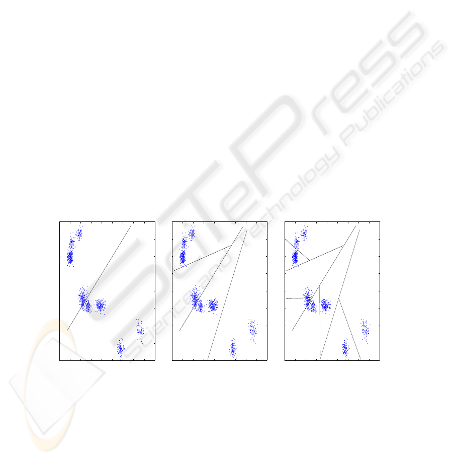
According to [4], in order to generate candidates, first we partition the dataset in M
subsets, one for each node as follows
X
j
= {(x, k) ∈ X, p(j|k, x) > p(i|k, x), ∀i 6= j}
Then employing the kd-tree partitioning method we repartition each X
j
in six subsets.
The statistics of the resulting subsets are probable estimates of µ
q
and σ
2
q
. The corre-
sponding estimation of prior is α
k
= p(j|k)/2. Partitioning each node we create 6M
sets of candidates θ
q
= {α
k
, µ
q
, σ
2
q
}, so we have to select the most appropriate accord-
ing to a criterion. Fig. 2 illustrates the partitioning stages for an artificial data set.
−1.5 −1 −0.5 0 0.5 1 1.5 2 2.5 3
−2
−1.5
−1
−0.5
0
0.5
1
1.5
2
−1.5 −1 −0.5 0 0.5 1 1.5 2 2.5 3
−2
−1.5
−1
−0.5
0
0.5
1
1.5
2
−1.5 −1 −0.5 0 0.5 1 1.5 2 2.5 3
−2
−1.5
−1
−0.5
0
0.5
1
1.5
2
Fig.2. Successive partitioning of an artificial dataset using the kd-tree method. All the 14 parti-
tions illustrated in the three graphs are considered to specify candidate parameter vectors.
We have already mentioned that we wish the new component to be placed at regions
in the data space containing examples of more than one class. A way to quantify the
7
degree to which a candidate component satisfies this property is to compute the change
of the log-likelihood for class k, caused by the addition of the candidate new component
q with density p(x; θ
q
). Thus, we compute the change of the log-likelihood ∆L
(q )
k
for
class k after the addition of q
∆L
(q )
k
=
1
N
k
(log ˆp(x|k) − log p(x|k)) =
1
N
k
X
x∈X
k
log
1 − α
k
(1 −
q(x)
p(x|k)
)
(10)
We retain those θ
q
that increase the log-likelihood of at least two classes and discard the
rest. For each retained θ
q
, we add the positive ∆L
q
k
terms to compute the total increase
of the log-likelihood ∆L
q
. The candidate q
⋆
whose value ∆L
q
⋆
is maximum is added
to the current network, if this maximum value is higher than a prespecified threshold
(set equal to 0.01 in all experiments). Otherwise, we consider that the attempt to add a
new node is unsuccessful.
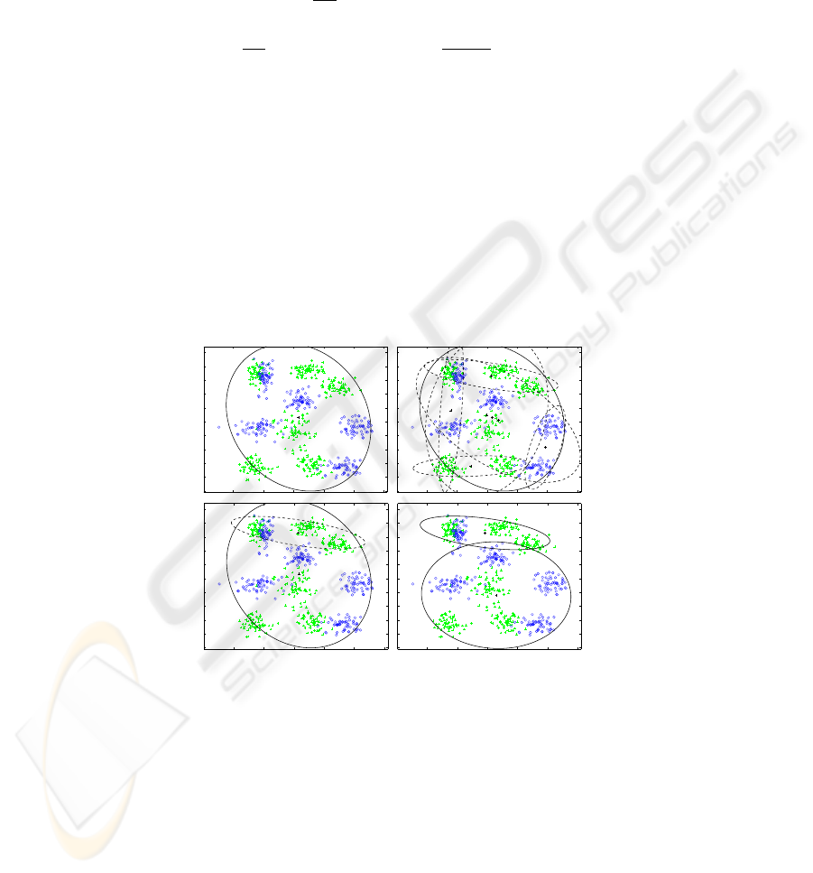
After the successful addition of a new node we apply the EM update equations to
the whole model with M + 1 components, as described in the previous section. This
procedure can be applied iteratively, in order to add a maximum number of nodes to the
given network. Figure 3 illustrates the addition of the first two network nodes.
0 0.2 0.4 0.6 0.8 1
0
0.1
0.2
0.3
0.4
0.5
0.6
0.7
0.8
0.9
1
0 0.2 0.4 0.6 0.8 1
0
0.1
0.2
0.3
0.4
0.5
0.6
0.7
0.8
0.9
1
0 0.2 0.4 0.6 0.8 1
0
0.1
0.2
0.3
0.4
0.5
0.6
0.7
0.8
0.9
1
0 0.2 0.4 0.6 0.8 1
0
0.1
0.2
0.3
0.4
0.5
0.6
0.7
0.8
0.9
1
Fig.3. Addition of the first two basis functions. The nodes of the network are depicted with solid
lines, and the candidate nodes with dotted lines.
2.2 Node Splitting
After the stage of adding nodes, there may be nodes of the network located to re-
gions with overlapping among classes. In order to increase the generalization per-
formance of the network we follow the approach suggested in [12], and split each
8

node. More specifically, we compute P (j|x, k) for every pattern x ∈ X, and check
if
P
x∈X
k
P (j|x, k) > 0 for more than one class k. If this happens, then we remove
it from the network, and add a separate component for each class. So finally every
subcomponent describes only one class. Splitting a component j, the resulting subcom-
ponent of class k is a Gaussian probability density function p(x|j, k), with mean µ
jk
,
variance matrix σ
2
jk
and mixing weight π
jk
. These parameters are estimated according
to:
π
jk
=
1
|X
k
|
X
x∈X
k
P (j|x, k) (11)
µ
jk
=
P
x∈X
k
P (j|x, k)x
P
x∈X
k
P (j|x, k)
(12)
σ
2
jk
=
P
x∈X
k
P (j|x, k)|x − µ
jk
|
2
P
x∈X
k
P (j|x, k)
(13)
After splitting the class conditional density is
p(x|k) =
M
X
j=1
π
jk
p(x|j, k), k = 1, . . . , K (14)
Using the above equations, the components whose region of influence contains sub-
regions with data of different classes, are split into class-specific subcomponents. The
parameters of each subcomponent are determined by the data of the respective class that
belong to the region of the component (i.e. they have high posterior value). As shown
in [12], the class conditional likelihood is increased for all classes after performing the
above splitting process.
3 Active Learning
In the previous section we described an incremental algorithm for training a PRBF
network using labeled data. In the following we incorporate the algorithm in an active
learning method, where we iteratively select unlabeled points from an available pool
of unlabeled points and ask for their labels. After the labels are given, the new points
are added in the labeled set and the network is trained again. The incremental training
algorithm presented in the previous section is particularly suited for such a learning
task, since it can naturally handle additional information in the training by adding new
nodes to the network in case this is necessary. Otherwise the whole learning procedure
should be applied from scratch.
The crucial issue in active learning is to select the unlabeled points that are benefi-
cial to the training of our classifier. We propose the selection of a point that lies near the
classification boundary. In this way we facilitate the iterative addition of basis functions
on the classification boundary, as described in the previous section.
As a criterion of selecting a suitable point we propose the ratio of class posteriors
as estimated by the current PRBF model. Let X
U
denote the set of unlabeled points and
9

X
L
the set of labeled points (X
U
∪ X
L
= X). For each unlabeled observation x ∈ X
U
we compute the class posterior p(k|x) for every class, and then find the two classes with
the largest posterior values:
κ
(x)
1
= arg max
k
p(k|x), κ
(x)
2
= arg max
k6=κ
(x)
1
p(k|x). (15)
We choose to ask for the label of ˆx that exhibits the smallest ratio of largest class
posteriors (3):
ˆx = arg min
x∈X
U
log
p(κ
(x)
1
|x)
p(κ
(x)
2
|x)
. (16)
In this way we pick the unlabeled observation that lies closer to the decision boundary
of the current classifier. Note that according to Bayes rule, we classify observations
to the class with the maximum class posterior (3). Thus for some x on the decision
boundary holds that p(κ
(x)
1
|x) = p(κ
(x)
2
|x). Consequently if an observation approaches
the decision boundary between two classes, then the corresponding logarithmic ratio of
class posteriors tends to zero.
Summarizing the presented methodology, we propose the following active learning
algorithm:
1. Input: The set X
L
of labeled observations, the set X
U
of unlabeled observations,
and a degenerate network P RBF
J=1
with one basis function. Let also X
L
= X
T
∪
X
V
where X
T
the training set and X
V
the validation set respectively.
2. For s = 0, . . . , S − 1
(a) Using training set X
T
, add one node to the network P RBF
J+s
to form
P RBF
J+s+1
.
3. For s = 0, . . . , S
(a) Using training set X
T
, split the nodes of P RBF
J+s
to form P RBF
split
J+s
.
4. Select the network P RBF
split
J
⋆
in {P RBF
split
J
, . . . , P RBF
split
J+S
} that achieves
highest classification accuracy on the validation set X
V
.
5. Set the current network: P RBF
J
= PRBF
split
J
⋆
.
6. If X
U
is empty or a maximum number of iterations is reached then terminate, else
(a) Pick a set X
A
of unlabeled observations ˆx according to (16), and for each ˆx
ask for its label ˆy.
(b) Update the sets: X
L
= X
L
∪ X
A
and X
U
= X
U
\ X
A
. Add half of the points
of X
A
to the training set X
T
and the other half to the validation set X
V
.
(c) Go to step 2.
In all our experiments we use S = 3, and the number of unlabeled points selected at
each iteration was equal to 10 with half of them added to the training set and the other
half to the validation set. The labeled set X
L
was initialized with 50 randomly selected
data points equally distributed among classes.
10
4 Experiments
For the experimental evaluation of our method we used three large multiclass data sets,
available from the UCI repository. The first is the satimage dataset that consists of 6435
data points with 36 continuous features and 6 classes. The second is the segmentation
set, that consists of 2310 points with 19 continuous features and 7 classes. The third is
the waveform set, that consists of 5000 points with 21 continuous features and 3 classes.
In all experiments we applied our algorithm starting with 20 randomly selected labeled
points, and actively selected 20 points at each iteration.
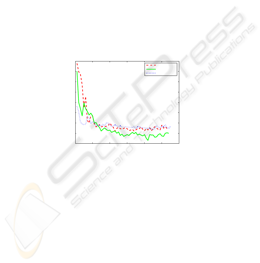
Figure 4 illustrates the generalization error as a function of active learning iterations.
It can be observed that in all cases the generalization error decreases very rapidly in the
initial iterations after the addition of a few labeled points. After the addition of about
500 points the error had reached a low value, and the addition of more points offers
slight improvement.
0 10 20 30 40 50 60
0
0.1
0.2
0.3
0.4
0.5
0.6
0.7
0.8
iterations
test error
satimage
segmentation
waveform
Fig.4. The generalization error using pool-based active PRBF learning on three UCI multiclass
datasets (satimage, segmentation and waveform).
5 Conclusions
We have proposed a pool-based active learning methodology for the Probabilistic RBF
classifier. We have exploited a recently proposed incremental training algorithm that
sequentially adds nodes to the network. Due to the incremental nature of this algorithm,
training does not start from scratch when new labeled data are added to the training set
and the method fits perfectly to the active learning framework. To select the unlabeled
data to be added to the labeled set, we used a criterion that estimates the class con-
ditional densities for the unlabeled data and prefers those points that lie closer to the
decision boundary. Experimental results on three large UCI datasets indicate that the
proposed active learning method works sufficient well.
11

References
1. Bishop, C. M. (1995). Neural Networks for Pattern Recognition. Oxford University Press.
2. Castelli, V. and Cover, T. (1995). On the exponential value of labeled samples. Pattern
Recognition Letters, 16:105–111.
3. Cohn, D., Ghahramani, Z., and Jordan, M. (1996). Active learning with statistical models.
Journal of Artificial Inteligence Research, 4:129–145.
4. Constantinopoulos, C. and Likas, A. (2006). An incremental training method for the proba-
bilistic RBF network. IEEE Trans. Neural Networks, to appear.
5. Dempster, A., Laird, N., and Rubin, D. (1977). Maximum likelihood estimation from in-
complete data via the EM algorithm. Journal of the Royal Statistical Society, Series B,
39(1):1–38.
6. Freund, Y., Seung, H. S., Shamir, E., and Tishby, N. (1997). Selective sampling using the
query by comitee algorithm. Machine Learning, 28:133–168.
7. McCallum, A. K. and Nigam, K. (1998). Employing EM in pool-based active learning for
text classification. In Shavlik, J. W., editor, Proc. 15th International Conference on Machine
Learning. Morgan Kaufmann.
8. McLachlan, G. and Krishnan, T. (1997). The EM algorithm and extensions. John Wiley &
Sons.
9. McLachlan, G. and Peel, D. (2000). Finite Mixture Models. John Wiley & Sons.
10. Titsias, M. K. and Likas, A. (2000). A probabilistic RBF network for classification. In Proc.
International Joint Conference on Neural Networks 4, pages 238–243. IEEE.
11. Titsias, M. K. and Likas, A. (2001). Shared kernel models for class conditional density
estimation. IEEE Trans. Neural Networks, 12(5):987–997.
12. Titsias, M. K. and Likas, A. (2002). Mixture of experts classification using a hierarchical
mixture model. Neural Computation, 14(9):2221–2244.
13. Titsias, M. K. and Likas, A. (2003). Class conditional density estimation using mixtures with
constrained component sharing. IEEE Trans. Pattern Anal. and Machine Intell., 25(7):924–
928.
14. Zhu, X., Lafferty, J., and Ghahramani, Z. (2003). Combining active learning and semi-
supervised learning using Gaussian fields and harmonic functions. In Proc. 20th Interna-
tional Conference on Machine Learning.
12
