
TRAJECTORY CONTROL AND MODELLING OF AN
OMNI-DIRECTIONAL MOBILE ROBOT
Andr
´
e Scolari Conceic¸
˜
ao, A. Paulo Moreira, Paulo J. Costa
Department of Electrical and Computer Engineering
University of Porto - Porto - Portugal.
Keywords:
Trajectory control, modelling and simulation, omni-directional mobile robot.
Abstract:
This paper presents a trajectory controller for an omni-directional mobile robot. The controller presents im-
portant features, as the possibility of defining different translation velocities and angular positions to the robot
during the trajectory following. The parameters of the controller are optimizated based on trajectory following
simulations, with the mobile robot model. Simulation and real results of trajectory following are presented.
1 INTRODUCTION
Omni-directional mobile robots have the ability to
move simultaneously and independently in translation
and rotation (Pin and Killough, 1994). However, non-
linearities, like motor dynamic constraints, and oth-
ers characteristics like friction, inertia moment and
mass of the robot, should be modelled, because can
greatly affect the robot behaviour. Hence, dynamic
modelling of mobile robots is very important to de-
sign of controllers, as in (Liu et al., 2003)(Watanabe,
1998)(Fraga et al., 2005), mainly when the robots
need to follow trajectories at higher velocity, with
sudden change in its direction and orientation.
The suggested controller presents interesting fea-
tures to follows the path correctly, how the possibility
to define different linear velocities and angular posi-
tions to the robot during the trajectory following. A
trajectory can be approximated with line segments. A
line segment has two distinct endpoints. We use in
this paper the name of a line segment with endpoints
A and B as ”line segment
AB”. Hence, we can define
linear velocities and angular position to the robot in
each endpoint of the line segment, moreover we can
adjust its velocities and angular position to the long
of the line segment. Another feature of the controller
is low computational time, which is essential in real
time applications.
The optimization of the parameters of the controller
is based on robot model. Due to values of time and er-
rors of position and orientation of the robot, in trajec-
tory following simulations with the robot model, we
can calculate the best parameters to the controller.
We focus attention on a omni-directional mobile
robot with four motors, as shown in Fig.1, built for
the 5dpo Robotic Soccer team from the Department
of Electrical and Computer Engineering at the Univer-
sity of Porto at Porto, Portugal(Moreira et al., 1999).
The organization of the paper is as follows. In sec-
tion 2, the omni-directional mobile robot model is de-
veloped. The controller for trajectory following is
presented in section 3. In section 4, the optimiza-
tion of the controller parameters, simulation results
and real results are presented. Finally, the conclusion
is drawn in section 5.
2 THE MOBILE ROBOT MODEL
The omni-directional mobile robot model is develo-
ped based on the dynamics, kinematics and DC mo-
tors of the robot.
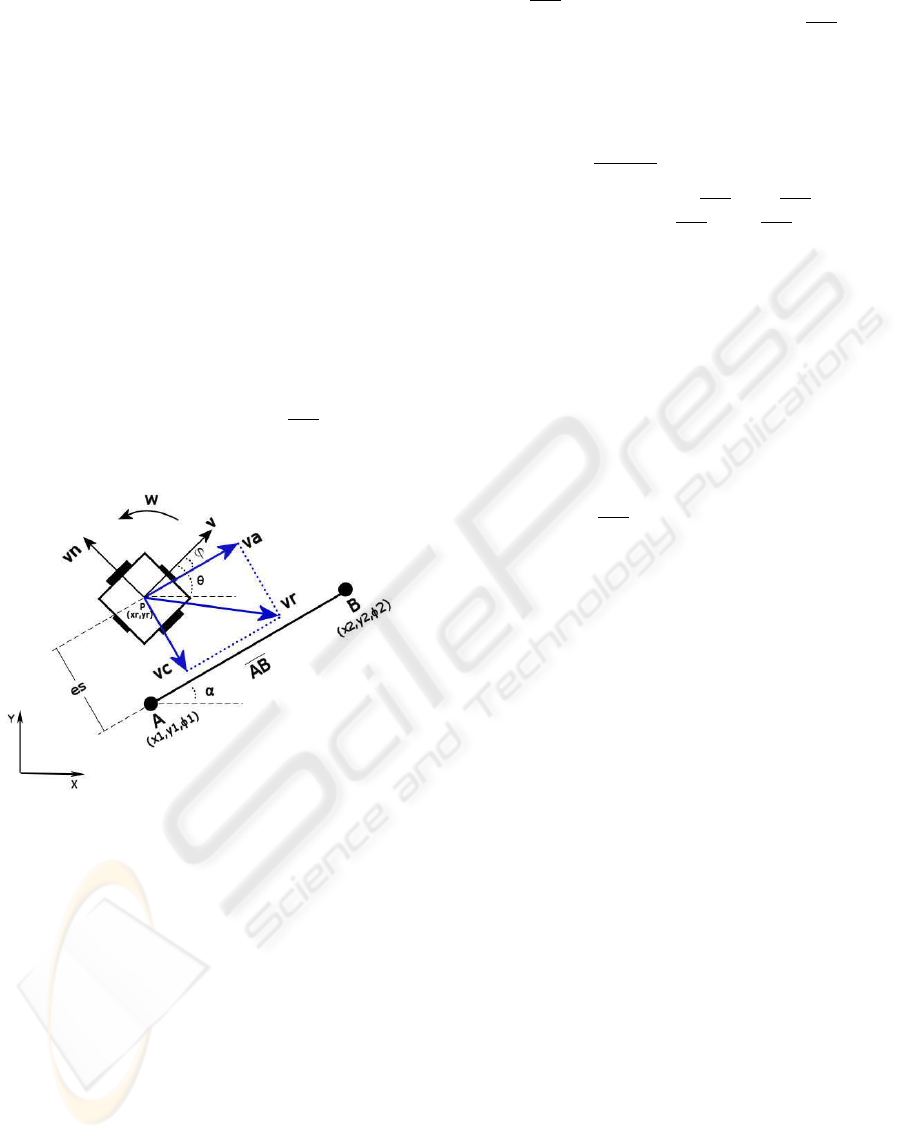
The World frame (X, Y, θ), the robot’s body frame
and the geometric parameters is shown in Fig. 2.
The following symbols, in SI unit system, are used
to modelling:
• b [m] → distance between the point P(center of
chassis) and robot’s wheels
• M [kg] → robot mass
• r [m] → wheel radius
• l → motor reduction
• J [kg.m
2
] → robot inertia moment
412
Conceição A., Moreira A. and Costa P. (2006).
TRAJECTORY CONTROL AND MODELLING OF AN OMNI-DIRECTIONAL MOBILE ROBOT.
In Proceedings of the Third International Conference on Informatics in Control, Automation and Robotics, pages 412-417
DOI: 10.5220/0001220904120417
Copyright
c
SciTePress
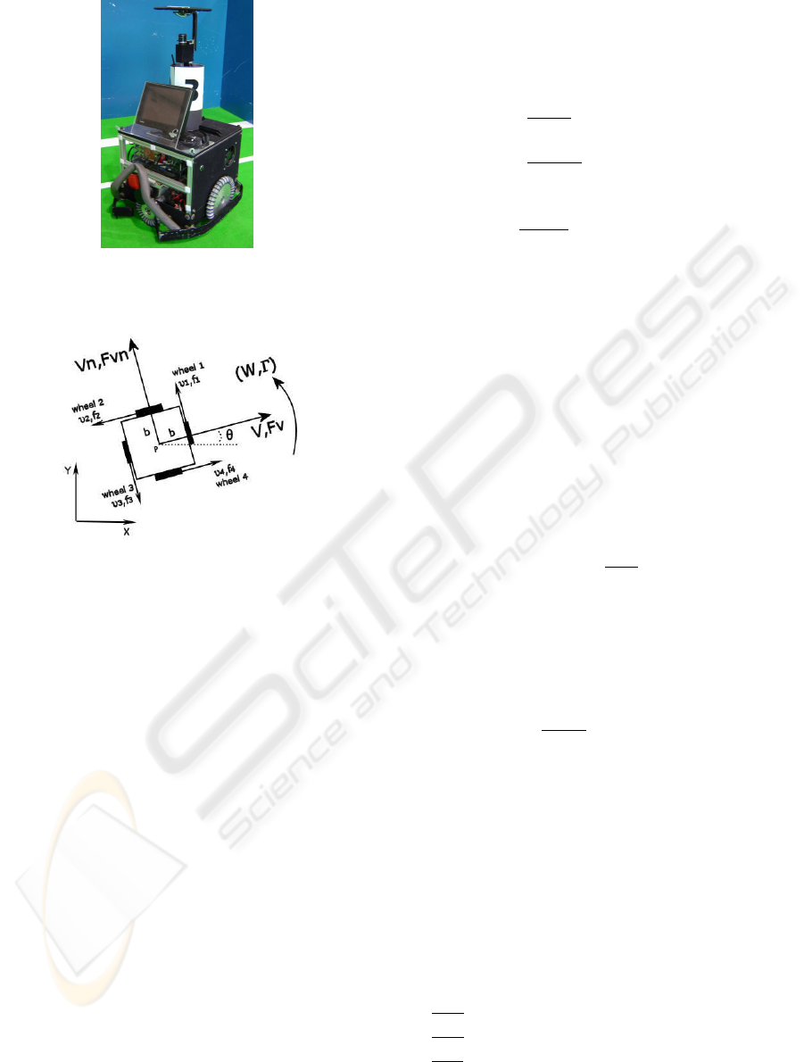
Figure 1: Mobile robot.
Figure 2: Geometric parameters and coordinate frames.
• B
v
, B
v n
[N/(m/s)] → viscous friction related to
V and V
n
velocities
• B
w
[N/(rad/s)] → viscous friction related to W
velocity
• C
v
, C
v n
[N] → coulomb friction related to V and
V
n
velocities
• V, V
n
[m/s] → linear velocities of the robot
• W [rad/s] → angular velocity of the robot
• θ [rad] → orientation angle of the robot
• F
v
, F
v n
[N] → traction forces of the robot
• Γ [N.m] → rotation torque of the robot
• v
1
, v
2
, v
3
, v
4
[m/s] → wheels linear velocities
• f
1
, f
2
, f
3
, f
4
[N] → wheels traction forces
• T
1
, T
2
, T
3
, T
4
[N.m] → wheels rotation torque
2.1 Robot Dynamics
By Newton’s law of motion and the robot’s body
frame, in Fig. 2, we have
F
v
(t) = M
dV (t)
dt
+ B
v
V (t) + C
v
sgn(V (t)) (1)
F
v n
(t) = M
dV n(t)
dt
+ B
v n
V
n
(t) + C
v n
sgn(V
n
(t))
(2)
Γ(t) = J
dW (t)
dt
+ B
w
W (t) + C
w
sgn(W(t)) (3)
where,
sgn(α) =
(
1, α > 0,
0, α = 0,
−1, α < 0.
The relationships between the robot’s traction
forces and the wheel’s traction forces are,
F
v
(t) = f
4
(t) − f
2
(t) (4)
F
v n
(t) = f
1
(t) − f
3
(t) (5)
Γ(t) = (f
1
(t) + f
2
(t) + f
3
(t) + f
4
(t))b (6)
The wheel’s traction force(f ) and the wheel’s
torque(T ), for of each DC motor, is as follow:
f(t) =
T (t)
r
(7)
T (t) = l.K
t
.i
a
(t) (8)
where i
a
(t) is the armature current and K
t
is motor
torque constant. The dynamics of each DC motor can
be described using the following equations,
u(t) = L
a
di
a
(t)
dt
+ R
a
i
a
(t) + K
v
w
m
(t) (9)
T (t) = K
t
i
a
(t) (10)
where L
a
is the armature inductance, R
a
is the ar-
mature resistance, u(t) is the applied armature vol-
tage, w
m
(t) is the rotor angular velocity in rad/sec,
k
v
is the emf constant.
2.2 Robot Kinematics
By geometric parameters of the robot and the robot’s
body frame, in Fig. 2, is possible to derive the motion
equations,
dx(t)
dt
= V (t)cos(θ(t)) − V n(t)sen(θ(t))
dy (t)
dt
= V (t)sen(θ(t)) + V n(t)cos(θ(t))
dθ(t)
dt
= W (t)
(11)
The relationships between wheel’s linear velocities
(v
1
, v
2
, v
3
and v
4
) and robot velocities (V ,V n and
TRAJECTORY CONTROL AND MODELLING OF AN OMNI-DIRECTIONAL MOBILE ROBOT
413
W ) are,
v
1
(t) = V
n
(t) + bW (t)
v
2
(t) = −V (t) + bW (t)
v
3
(t) = −V
n
(t) + bW (t)
v
4
(t) = V (t) + bW (t)
(12)
Where x(t) and y(t) is the localization of the point
P , and θ(t) the orientation angle of the robot.
3 LINE SEGMENT
CONTROLLER
The proposed controller adjusts the position and ori-
entation of the robot to follow a line segment, defined
in the plane XY , as shown in Fig.3. From a line seg-
ment and the position of the robot, we can define the
velocity vectors to the robot. The velocity vectors,
robot position(P ) and a line segment(AB) are shown
in Fig.3. The robot position is P (x
r
, y
r
) and θ is the
Figure 3: Schematic of the controller.
orientation angle of the robot in the plane XY . The
velocity vectors V and V n are perpendicular, and re-
present the linear velocities of the robot. The angu-
lar velocity of the robot is W . The angle ϕ is the
difference between the line segment angle (α) and the
robot angle (θ):
ϕ = α − θ. (13)
The velocity vector v
r
is the desired linear velocity
to robot, called too reference velocity. The velocity
v
r
can receive different values in both points(A and
B) of the line segment, hence the robot can follow
trajectories with different reference velocities. The
reference velocity to the long of the line segment is:
v
r
= v
r1
(1 − d) + v
r2
d. (14)
Where v
r1
is the reference velocity of the point A and
v
r2
is the reference velocity of the point B, of the line
segment AB. The variable d is the projection from
robot position(P (xr, yr)) to line segment
AB, it is
normalized to length of the line segment. The vector
velocities of the controller, are as follow:
v
c
= e
s
k
1
, (15)
v
a
=
0 , v
2
r
− v
2
c
< 0,
p
v
2
r
− v
2
c
, v
2
r
− v
2
c
> 0.
(16)
With the vector v
a
parallel to
AB(v
a
|| AB) and the
vector v
c
perpendicular to
AB(v
c
⊥ AB). The dis-
tance between the robot and the line segment is e
s
,
and k
1
is a gain. We can calculate the vector veloci-
ties V and V
n
, using a rotation matrix:
V
V n
=
cos(ϕ) −sen(ϕ)
sen(ϕ) cos(ϕ)
v
a
v
c
.
The robot angular velocity(W ) is calculated based
on robot angular position(θ) and desired angular
positions(φ) in both points(A and B) of the line seg-
ment. For all line segment, the angular velocity W
is calculated with a similar variation used in equa-
tion 14, in function of d. Therefore, when is defined
the line segment
AB, we define the desired angular
positions(φ
1
and φ
2
) in each point of the line segment.
The controller to robot angular position is defined as
follow:
W = e
θ
k
2
. (17)
with:
e
θ
= θ
ref
− θ, (18)
θ
ref
= φ
1
(1 − d) + φ
2
d. (19)
where k
2
is a gain, e
θ
is the error between desired
angular position(θ
ref
) and robot angular position(θ).
4 OPTIMIZATION OF THE
CONTROLLER
After we define the controller structure, we need to
choose the appropriate values to gain k
1
and gain k
2
.
A cost function (C) was created to measure the per-
formance of trajectory following. The cost function is
described as follow:
C(k
1
, k
2
) = E
d
P
d
+ E
a
P
a
+ (T
r
− T
i
)P
t
.
Where:
E
d
֒→ Mean square error(MSE) related to e
s
, for all
trajectory following;
E
a
֒→ Mean square error related to e
θ
, for all trajec-
tory following;
T
i
֒→ ideal time to follow the trajectory;
T
r
֒→ robot time to follow the trajectory;
ICINCO 2006 - ROBOTICS AND AUTOMATION
414
P
d
, P
a
, P
t
֒→ gain related to errors.
We used the robot model, described in section 2, to
define k
1
and k
2
gains. Trajectory following simula-
tions, see Fig. 4, with different values of the k
1
and
k
2
, make possible obtain the values of the cost func-
tion. The objective is found the values of the k
1
and
k
2
that result the minimum value of the cost function.
Through real experiments with the robot, we know
that gains (k
1
and k
2
) above of 15 do not cause effect
in trajectory following, due to saturation of the actu-
ators. Hence, we used values between 0 and 20, with
resolution of 0.5 in trajectory following simulations.
The trajectory following simulations were made for 3
values of the linear velocity v
r
: 1, 0.7 e 0.4 [m/s].
So, it computed 1600 simulations for each velocity,
resulting in 4800 total simulations. Without the robot
model, it will be impossible. Furthermore, the total
simulation time for each velocity(1600 simulations)
is about 10 seconds, therefore we did not need to use
minimization algorithms.
The trajectory used in the simulations has special
features, as sudden change of direction and orienta-
tion to the robot, in order to test the controller in hard
condition. The Fig. 4 shows the trajectory used in
the simulations, with the points(x,y). The Fig. 5
shows values of the desired angular positions(φ) for
each point(x
i
,y
i
), i=1, ...13 of the trajectory.
0 0.5 1 1.5 2 2.5 3
−0.2
0
0.2
0.4
0.6
0.8
1
1.2
1.4
1.6
1.8
X[m]
Y[m]
Figure 4: Trajectory to calculate the cost function.
0 2 4 6 8 10 12 14
−2
−1.5
−1
−0.5
0
0.5
1
1.5
2
i
Teta[rad]
Figure 5: Angular positions(φ) of the trajectory.
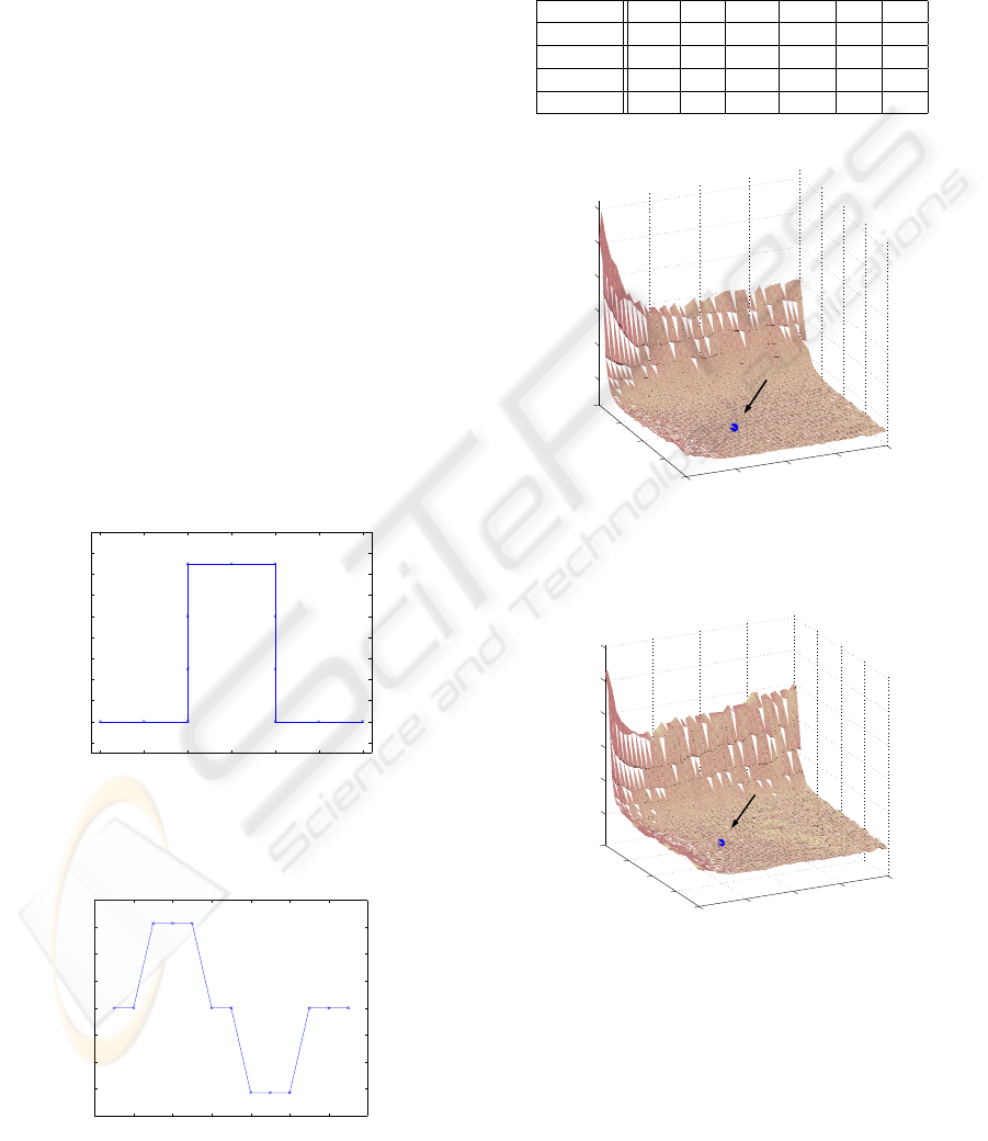
The cost functions for 3 linear velocities v
r
and the
gains (k
1
and k
2
) are shown in Figs. 6, 7 and 8. The
minimum values of the cost function(C) and corres-
pondents gains are shown in table 1. The values of
Table 1: Minimum values of the cost function.
v
r
[m/s] C k
1
k
2
P
d
P
a
P
t
1 5.57 8 12.5 1000 10 1
0.7 3.87 7 10.5 1000 10 1
0.4 1.21 7.5 9 1000 10 0.5
mean≈ - 7.5 10.5 - - -
0
5
10
15
20
0
5
10
15
20
10
20
30
40
50
60
k1
k2
C
Figure 6: Cost function, v
r
= 1 m/s.
0
5
10
15
20
0
5
10
15
20
5
10
15
20
25
30
k1
k2
C
Figure 7: Cost function, v
r
= 0.7 m/s.
the gains P
d
, P
a
and P
t
were defined in order to be
even the values of the errors E
d
, E
a
and (T
r
− T
i
).
Currently we use the mean of the gains values, shown
in table 1. We tested this values in robot trajectory fol-
lowing for the linear velocities v
r
= 0.4, 0.7, 1[m/s].
It had a good performance so, the use of different
gains for different linear velocities is not necessary.
Real and simulated results with gain k
1
= 7.5, gain
TRAJECTORY CONTROL AND MODELLING OF AN OMNI-DIRECTIONAL MOBILE ROBOT
415
0
5
10
15
20
0
5
10
15
20
0
2
4
6
8
10
12
14
16
18
k1
k2
C
Figure 8: Cost function, v
r
= 0.4 m/s.
k
2
= 10.5 and linear velocity v
r
= 1[m/s] are shown
if Figs. 9, 10 and 11.
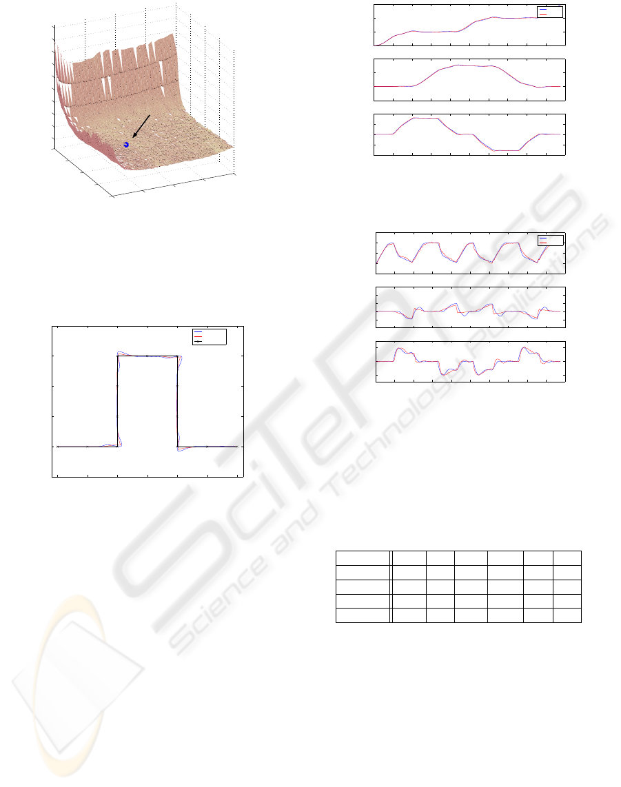
0 0.5 1 1.5 2 2.5 3
−0.5
0
0.5
1
1.5
2
X[m]
Y[m]
Simulation
Robot
Trajectory
Figure 9: Simulated and real trajectory.
The procedure to define the gains k
1
and k
2
was
repeated with a trajectory like ”8”, see Fig. 12(a),
this trajectory has a different feature than first one, in
Fig. 4. The robot does not need to do sudden change
of direction and orientation. The table 2 shows the
minimum values of the cost function(C) and corres-
pondents gains. In this simulations we kept the same
gains to P
d
, P
a
and P
t
, to get a comparison. The re-
sults for the gain k
2
were equal in both procedures.
The results for the gain k
1
were not equal, the gain
diminished with the reduction of the linear velocity
v
r
. It happened due to characteristics of the trajectory
”8”, this trajectory is more soft than the first trajec-
tory, consequently the error E
d
diminished too.
Finally, we tested the gains k
1
and k
2
obtained with
the first trajectory, in the robot to follow the trajec-
tory ”8”, the robot had a satisfactory performance.
We decided to use the bigger gains (k
1
= 7.5 and
k
2
= 10.5), because in robotic soccer application the
mobile robot needs to execute trajectories quickly and
with a perfect position to the objective, for example,
0 1 2 3 4 5 6 7 8 9 10
0
1
2
3
X
0 1 2 3 4 5 6 7 8 9 10
−1
0
1
2
Y
0 1 2 3 4 5 6 7 8 9 10
−2
−1
0
1
2
Teta
time[sec]
Sim
Robot
Figure 10: X(m), Y (m), θ(rad).
0 1 2 3 4 5 6 7 8 9 10
−0.5
0
0.5
1
1.5
V
0 1 2 3 4 5 6 7 8 9 10
−1
−0.5
0
0.5
1
1.5
Vn
0 1 2 3 4 5 6 7 8 9 10
−2
0
2
W
time[sec]
Sim
Robot
Figure 11: V (m/s), V n(m/s), W (rad/s).
positioning to the ball, or to the goal, or to avoid dy-
namic obstacles.
Table 2: Minimum values of the cost function, trajectory
”8”.
v
r
[m/s] C k
1
k
2
P
d
P
a
P
t
1 2.84 9 12.5 1000 10 1
0.7 0.72 5 10.5 1000 10 1
0.4 0.22 3 9 1000 10 0.5
mean≈ - 5.5 10.5 - - -
5 CONCLUSION
In this paper, a controller for trajectory following has
been presented. The proposed controller presents im-
portant features, as the possibility of defining differ-
ent translation velocities and angular positions to the
robot during the trajectory following. Besides, it does
not demand a high computational time, which is es-
sential in real time applications and applications of
high velocity. The robot model was essential to opti-
mization of the parameters of the controller.
ICINCO 2006 - ROBOTICS AND AUTOMATION
416
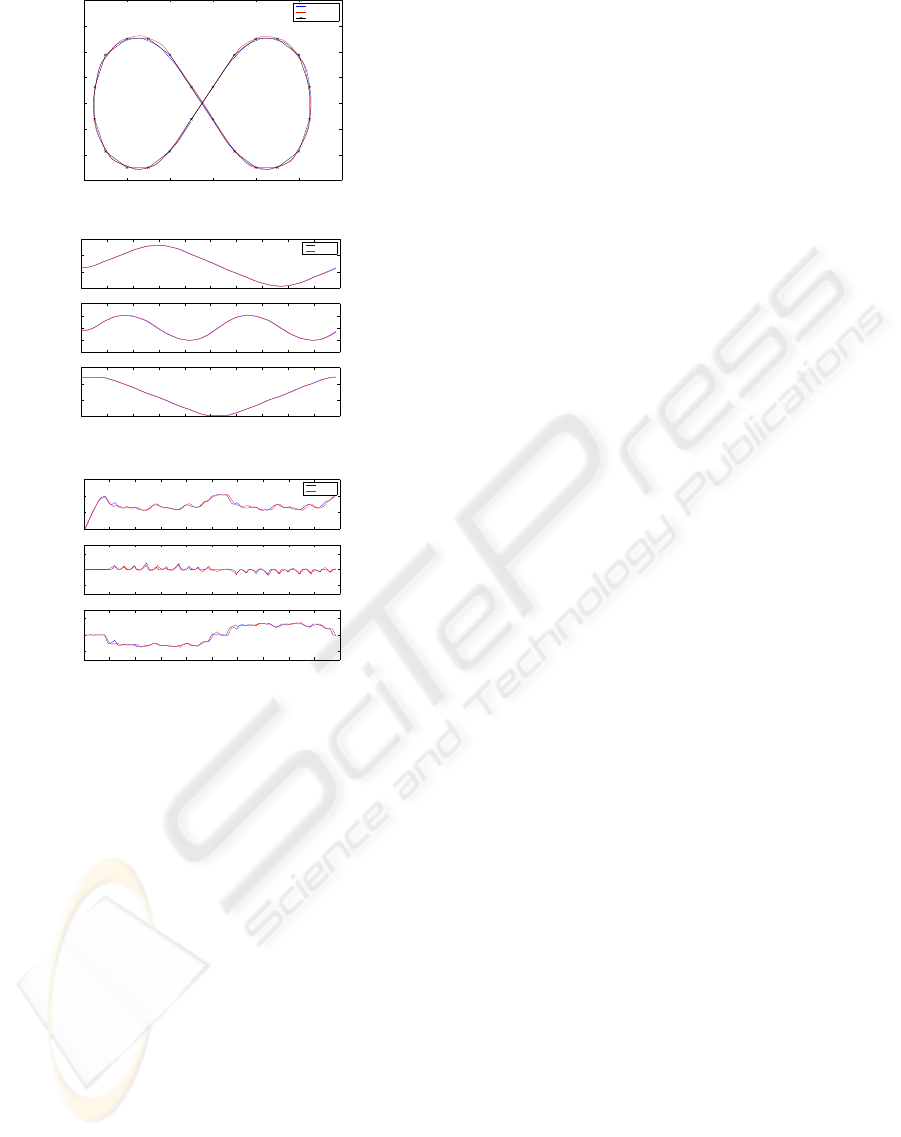
0 0.5 1 1.5 2 2.5 3
−0.4
−0.2
0
0.2
0.4
0.6
X[m]
Y[m]
Simulation
Robot
Trajectory
(a) Simulated and real trajectory.
0 1 2 3 4 5 6 7 8 9 10
0
1
2
3
X
0 1 2 3 4 5 6 7 8 9 10
−1
−0.5
0
0.5
1
Y
0 1 2 3 4 5 6 7 8 9 10
−4
−2
0
2
Teta
Time[sec]
Sim
Robot
(b) X(m), Y (m), θ(rad).
0 1 2 3 4 5 6 7 8 9 10
0
0.5
1
1.5
V
0 1 2 3 4 5 6 7 8 9 10
−0.5
0
0.5
Vn
0 1 2 3 4 5 6 7 8 9 10
−2
0
2
W
Time[sec]
Sim
Robot
(c) V (m/s), V n(m/s), W (rad/s).
Figure 12: Trajectory ”8”.
REFERENCES
Fraga, S. L., borges de Sousa, J., and Pereira, F. L. (2005).
Optimizao dinmica para planeamento de movimento e
controlo de veculos autnomos. Robtica 2005 - Festival
Nacional de Robtica.
Liu, Y., Wu, X., Zhu, J. J., and Lew, J. (2003). Omni-
directional mobile robot controller design by trajec-
tory linearization. Proceedings of the American Con-
trol Conference, 4:3423 – 3428.
Moreira, A., Costa, P., A.Sousa, Marques, P., Costa, P., and
Matos, A. (1999). 5dpo team description robocup.
Robot World Cup Soccer Games and Conference.
Pin, F. G. and Killough, S. M. (1994). A new family of om-
nidirectional and holonomic wheeled platforms for-
mobile robots. IEEE Transactions on Robotics and
Automation, 10:480–489.
Watanabe, K. (1998). Control of ominidirectional mobile
robot. 2nd Int. Conf. on Knowledge-Based Intelligent
Electronic Systems.
TRAJECTORY CONTROL AND MODELLING OF AN OMNI-DIRECTIONAL MOBILE ROBOT
417
