DYNAMIC PARAMETERS IDENTIFICATION OF AN

OMNI-DIRECTIONAL MOBILE ROBOT

Andr

e Scolari Conceic¸

ao, A. Paulo Moreira, Paulo J. Costa

Department of Electrical and Computer Engineering

University of Porto - Porto - Portugal.

Keywords:

Mobile robots, model and identiﬁcation systems, simulations.

Abstract:

This paper presents the experimental dynamic parameters identiﬁcation of an omni-directional mobile robot

with four wheels. Three methods of parameters identiﬁcation related to dynamic equations are described, the

parameters are the viscous frictions, the coulomb frictions and the inertia moment of the robot. A simulation

environment, simulation results and real results are presented.

1 INTRODUCTION

Dynamic modelling of mobile robots is very impor-

tant to design of controllers, mainly when the ro-

bots need to travel at higher velocity and perform

heavy works. For example, in (Liu et al., 2003)

and (Watanabe, 1998), control strategies for omni-

directional robots using the dynamic model are dis-

cussed. However, non-linearities, like motor dynamic

constraints can greatly affect the robot behaviour, es-

pecially when the robot is accelerated and deceler-

ated. This paper presents a robot model identiﬁca-

tion that could ﬁnd the non-linear saturation elements.

Three methods are described to identiﬁcation of the

model’s parameters.

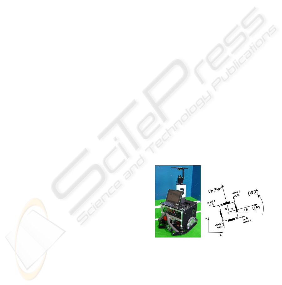
We focus attention on a omni-directional mobile

robot with four motors, as shown in Fig.1(a), built

for the 5dpo Robotic Soccer team from the Depart-

ment of Electrical and Computer Engineering at the

University of Porto at Porto, Portugal. For this ap-

plication (Robotic Soccer) the mobile robot needs to

execute trajectories quickly and with a perfect posi-

tion to the objective, for example, positioning to the

ball, or to the goal, or to avoid dynamic obstacles. So,

the dynamic characteristics of the motion are essential

to follows the path correctly.

In section 2, the omni-directional mobile robot

model is developed. The experimental methods of

identiﬁcation to model’s parameters is presented in

section 3. In section 4, simulation environment, simu-

lation and real results of the identiﬁed model are pre-

sented. Finally, the conclusion and future works are

drawn in section 5.

2 THE MOBILE ROBOT MODEL

The omni-directional mobile robot model is develo-

ped based on the dynamics, kinematics and DC mo-

tors of the robot.

(a) Mobile robot. (b) Geometric parameters

and coordinate frames.

Figure 1: Omni-Directional robot.

The World frame (X, Y, θ), the robot’s body frame

and the geometric parameters are shown in Fig. 1(b).

The following symbols, in SI unit system, are used to

modelling:

• b [m] → distance between the point P(center of chassis)

and robot’s wheels

565

Conceição A., Moreira A. and Costa P. (2006).

DYNAMIC PARAMETERS IDENTIFICATION OF AN OMNI-DIRECTIONAL MOBILE ROBOT.

In Proceedings of the Third International Conference on Informatics in Control, Automation and Robotics, pages 565-570

DOI: 10.5220/0001220805650570

 SciTePress

• M [kg] → robot mass

• r [m] → wheel radius

• l → motor reduction

• J [kg.m

] → robot inertia moment

• B

, B

[N/(m/s)] → viscous friction related to V

and V

velocities

• B

[N/(rad/s)] → viscous friction related to W velo-

city

• C

, C

[N] → coulomb friction related to V and V

velocities

• C

[N.m] → coulomb friction related to W velocity

• V, V

[m/s] → linear velocities of the robot

• W [rad/s] → angular velocity of the robot

• θ [rad] → orientation angle of the robot

• F

, F

[N] → traction forces of the robot

• Γ [N.m] → rotation torque of the robot

• v

, v

[m/s] → wheels linear velocities

• f

, f

[N] → wheels traction forces

• T

, T

[N.m] → wheels rotation torque

2.1 Robot Dynamics

By Newton’s law of motion and the robot’s body

frame, in Fig. 1(b), we have

(t) = M

dV (t)

+ B

V (t) + C

sgn(V (t)) (1)

(t) = M

dV n(t)

+ B

(t) + C

sgn(V

(t))

(2)

Γ(t) = J

dW (t)

+ B

W (t) + C

sgn(W (t)) (3)

where,

sgn(α) =

(

1, α > 0,

0, α = 0,

−1, α < 0.

The relationships between the robot’s traction

forces and the wheel’s traction forces are,

(t) = f

(t) − f

(t) (4)

v n

(t) = f

(t) − f

(t) (5)

Γ(t) = (f

(t) + f

(t))b (6)

The wheel’s traction force(f) and the wheel’s

torque(T ), for of each DC motor, is as follow:

f(t) =

T (t)

(7)

T (t) = l.K

(t) (8)

where i

(t) is the armature current and K

is motor

torque constant. The dynamics of each DC motor can

be described using the following equations,

u(t) = L

(t)

+ R

(t) + K

(t) (9)

T (t) = K

(t) (10)

where L

is the armature inductance, R

is the ar-

mature resistance, u(t) is the applied armature vol-

tage, w

(t) is the rotor angular velocity in rad/sec,

is the emf constant.

2.2 Robot Kinematics

By geometric parameters of the robot and the robot’s

body frame, in Fig. 1(b), it is possible to derive the

motion equations,

dx(t)

= V (t)cos(θ(t)) − V n(t)sen(θ (t))

dy ( t)

= V (t)sen(θ(t)) + V n(t)cos(θ(t))

dθ(t)

= W (t)

(11)

The relationships between wheel’s linear velocities

, v

and v

) and robot velocities (V ,V n and

W ) are,

(t) = V

(t) + bW (t)

(t) = −V (t) + bW (t)

(t) = −V

(t) + bW (t)

(t) = V (t) + bW (t)

(12)

Where x(t) and y(t) is the localization of the point

P , and θ(t) the orientation angle of the robot.

3 MODEL’S PARAMETERS

IDENTIFICATION

The parameters related to dynamic equations of the

mobile robot were experimentally identiﬁed. The

parameters are the viscous frictions (B

, B

v n

, B

the coulomb frictions (C

, C

v n

, C

) and the inertia

moment(J) of the mobile robot. The robot mass was

balanced(M = 35kg). Three methods were used

to identify the parameters, which are detailed in the

next subsections. The coulomb and viscous frictions

were identiﬁed with the methods 1 and 2. The inertia

moment was identiﬁed by two ways: combining the

method 1 with the method 2, and with the method 3.

Thus, we used two methods for identify the frictions(1

and 2) and two methods(1+2 and 3) for identify the

inertia moment.

3.1 Method 1 - Robot on Steady

State Velocity

This method was used to identify the viscous

frictions (B

, B

v n

, B

) and the coulomb frictions

ICINCO 2006 - ROBOTICS AND AUTOMATION

566

, C

v n

, C

) of the mobile robot. This method

consists of apply velocities V , V

and W in robot,

and measure the traction forces(F

, F

v n

) and the

torque(Γ), with the robot on steady state velocity. Due

to steady state velocity (null derivatives) and for posi-

tive velocities, we can simplify the equations 1, 2 and

(t) = B

V (t) + C

(13)

v n

(t) = B

v n

(t) + C

v n

(14)

Γ(t) = B

W (t) + C

(15)

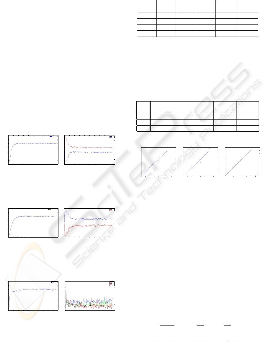
Three experiments had been made, for V , V

and

W separately. The experiment consists in apply four

velocities and measure the traction forces and the

torque. The table 1 shows the applied velocities and

the resulting forces and torque. The forces and torque

were calculated based in the motor’s currents, using

the set of equations 4...8. The velocities and cur-

rents of the ﬁrst, second and third experiments for

V = 1(m/s), V

= 1(m/s) and W = 1(rad/s),

are shown in Figs. 2, 3 and 4.

0 0.5 1 1.5 2 2.5 3 3.5 4 4.5 5

0.2

0.4

0.6

0.8

1.2

1.4

Speed V

time[sec]

V [m/s]

V=1 [m/s]

(a) V = 1 (m/s)

0 0.5 1 1.5 2 2.5 3 3.5 4 4.5 5

−6

−4

−2

Currents i2,i4

time[sec]

I[A]

(b) i

2, i

4 (A)

Figure 2: Velocity and currents - ﬁrst experiment.

0 0.5 1 1.5 2 2.5 3 3.5 4 4.5 5

0.2

0.4

0.6

0.8

1.2

1.4

Speed Vn

time[sec]

Vn [m/s]

Vn=1 [m/s]

(a) V n = 1 (m/s)

0 0.5 1 1.5 2 2.5 3 3.5 4 4.5 5

−6

−4

−2

Currents i1,i3

time[sec]

I[A]

(b) i

1, i

3 (A)

Figure 3: Velocity and currents - second experiment.

0 0.5 1 1.5 2 2.5 3 3.5 4 4.5 5

0.2

0.4

0.6

0.8

1.2

1.4

Speed W

time[sec]

W [rad/s]

W=1

(a) W = 1 (rad/s)

0 0.5 1 1.5 2 2.5 3 3.5 4 4.5 5

0.5

1.5

2.5

Currents i1,i2,i3,i4

time[sec]

I[A]

(b) i

1, i

2, i

3, i

4 (A)

Figure 4: Velocity and currents - third experiment.

Since we have the values for velocities and forces,

we can estimate the viscous and coulomb frictions.

Table 1: Applied velocities and resulting forces and torque.

V F

W Γ

(m/s) (N) (m/s) (N) (rad/s) (N.m)

0.6 30.585 0.6 30.285 0.6 5.556

0.8 31.459 0.8 30.814 0.8 5.730

1 31.874 1 31.174 1 5.842

1.2 32.765 1.2 32.106 1.2 6.009

The least-squares line method was used to approxi-

mate the set of data to a linear model(y = ax+ b). The

Fig. 5 shows the applied velocities, resulting forces

and the best ﬁtting line. The resulting equations and

the frictions are presented in the table 2.

Table 2: Resulting equations and frictions - method 1.

Equations B

V F

(t) = 3.45V (t) + 28.55 3.45 28.55

(t) = 2.90V

(t) + 28.46 2.90 28.46

W Γ(t) = 0.73W (t) + 5.12 0.73 5.12

0.6 0.7 0.8 0.9 1 1.1 1.2 1.3 1.4

30.5

31.5

32.5

V[m/s]

Fv[N]

(a) F

= f(V )

0.6 0.7 0.8 0.9 1 1.1 1.2 1.3 1.4

30.2

30.4

30.6

30.8

31.2

31.4

31.6

31.8

32.2

Vn[m/s]

Fvn[N]

(b) F

= f(V

)

0.6 0.7 0.8 0.9 1 1.1 1.2 1.3 1.4

5.55

5.6

5.65

5.7

5.75

5.8

5.85

5.9

5.95

6.05

W[rad/s]

T[Nm]

Figure 5: Forces and torque vs. velocities.

3.2 Method 2 - Robot with Null

Traction Forces

In this method, the velocity variation with null

traction forces was used to estimate the viscous

frictions(B

and B

v n

), the coulomb frictions (C

and

v n

) and the inertia moment J of the robot. Firstly,

a constant velocity was applied on the robot, and then

the robot motors were turned off, which resulted in

null currents and null forces, consequently, provoking

a velocity decrease until the robot stopped.

From the equations 1, 2 and 3 with null forces and

null torque, we have the following equations for posi-

tive velocities:

dV (t)

= −

V (t) −

(16)

dV n(t)

= −

v n

(t) −

v n

(17)

dW (t)

= −

W (t) −

(18)

DYNAMIC PARAMETERS IDENTIFICATION OF AN OMNI-DIRECTIONAL MOBILE ROBOT

567

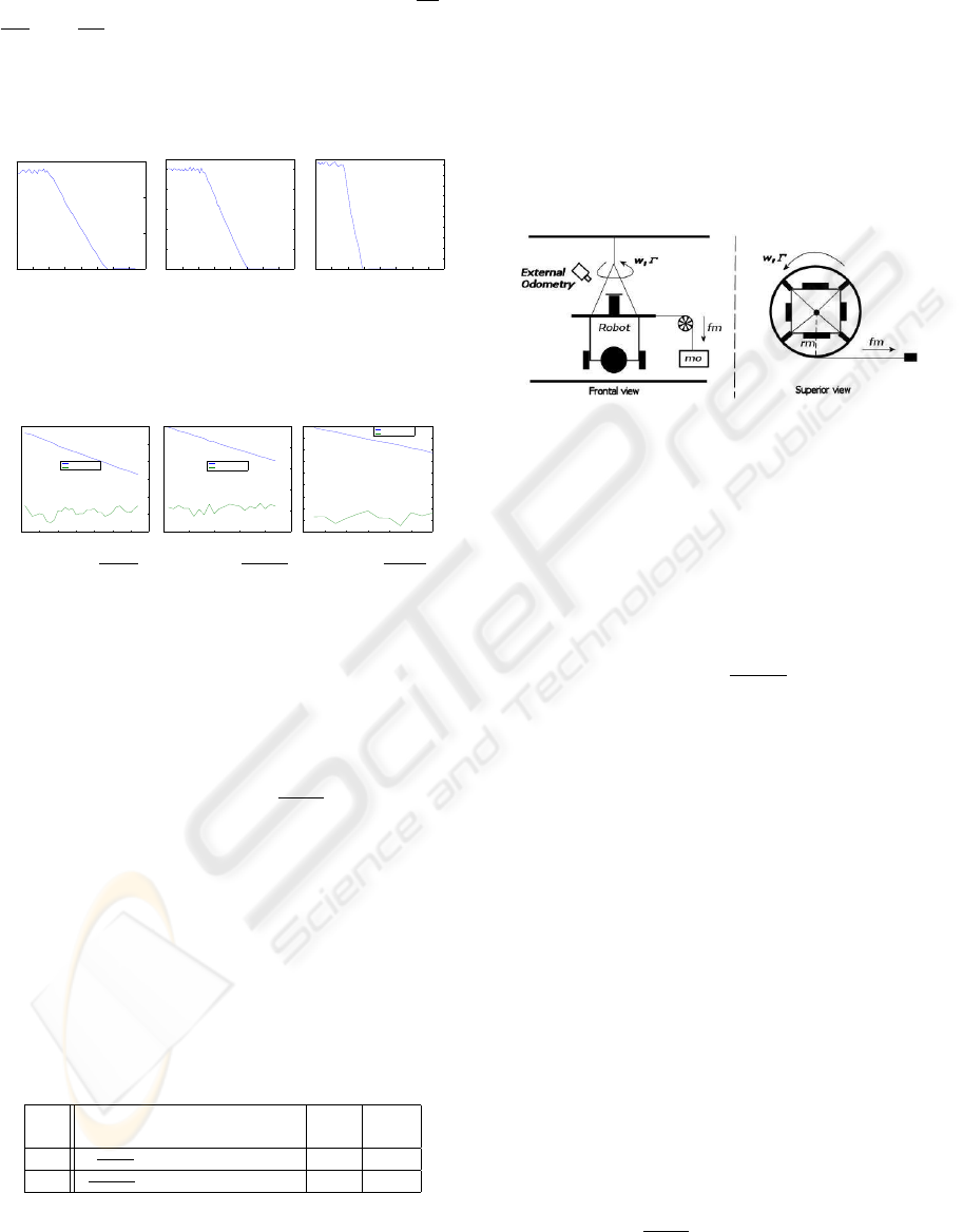
Three experiments had been made, for V , V

and

W separately, see Fig. 6. The accelerations(

and

) were calculated from the velocities(V ,

and W ), using the Euler’s method(Franklin et al.,

1997)). We used the range of data, where the forces

and torque were null to estimate the parameters, as in

Fig.7.

0 10 20 30 40 50 60 70 80

0.5

1.5

V[m/s]

Samples

(a) V (t)(m/s)

0 10 20 30 40 50 60 70 80

0.2

0.4

0.6

0.8

Vn[m/s]

Samples

(b) V

(t)(m/s)

0 10 20 30 40 50 60 70 80

0.2

0.4

0.6

0.8

1.2

1.4

1.6

1.8

W[rad/s]

Samples

Figure 6: Velocities behaviour.

0 5 10 15 20 25 30 35

−1.5

−1

−0.5

0.5

1.5

Samples

Velocity [m/s]

Acceleration[m/s.s]

(a) V (t),

dV (t)

0 5 10 15 20 25

−1.5

−1

−0.5

0.5

Samples

Velocity[m/s]

Acceleration[m/s.s]

(b) V

(t),

(t)

0 2 4 6 8 10 12

−6

−5

−4

−3

−2

−1

Samples

Velocity[rad/s]

Aceleration[rad/s.s]

dW (t)

Figure 7: Velocities and accelerations.

In order to estimate the viscous and the coulomb

frictions, the mass M and the inertia moment J

values are necessary. As there is no inertia mo-

ment J value, an estimation of J was ﬁrstly ob-

tained. We used the equation 18, the velocity curve

W (t) and the acceleration curve

dW (t)

shown in Fig.

7(c). The viscous(B

) and the coulomb(C

) fric-

tions, estimated with method 1, were used on equa-

tion 18. The estimated robot inertia moment was

J = 1.358[kg.m

Since we have the values of robot mass, velo-

city and acceleration, we can apply on equations 16

and 17, to obtain viscous frictions(B

and B

v n

) and

coulomb frictions (C

and C

v n

). The table 3 shows

the equations obtained through least-squares method

and the friction values.

Table 3: Resulting equations and frictions - method 2.

Equations B

, C

dV (t)

= −0.11V (t) − 0.86

4.01 30.35

dV n(t)

= −0.10V

(t) − 0.87

3.77 30.76

3.3 Method 3 - Inertia Moment

Identiﬁcation

A practical method for estimating the moment of iner-

tia J of the robot, to compare with the estimation

of the methods 1+2, is presented. The robot was

hanged from the ceiling by wire, see ﬁgure 8, to eli-

minate frictions between the robot and the ﬂoor. The

mass(m

) was hanged at the disc attached to the ro-

bot, by a wire.

Figure 8: Schematic of the experience.

By applying a known torque(Γ(t)) to robot body,

and measuring the resultant angular position(θ(t)), by

a external odometry system based on vision, we can

compute the moment of inertia of the robot. Based

in rotational equation of motion, see equation 3, and

considering null friction values (B

e B

), we get:

Γ(t) = J

dW (t)

(19)

The torque Γ(t) and the applied force f

(t) are

Γ(t) = f

(t)r

(20)

(t) = m

g (21)

where g is the acceleration of gravity (≈

9.8[m/s

]), m

is the mass and r

is the radius

disc(0.25[m]).

Four experiments had been made to identify the

value of J. The experiments 1, 2 and 3 were per-

formed with an object with mass equal 0.510 Kg, and

the experiment 4 with a object with mass equal 1 Kg.

Our objective was to verify the repeatability of the ex-

periments.

The ﬁgure 9(a) shows the angular position (θ(t))

curve for the ﬁrst experiment. The angular velocities

(W (t)) were calculated using the derivative of the an-

gular position. The ﬁgure 9(b) shows the angular ve-

locity and the best ﬁtting line to the angular velocity,

calculated by least-squares line method, that give us

the value of the angular accelerations.

The table 4 shows the torque values(Γ), angu-

lar accelerations(

dW (t)

) and inertia moments(J) ob-

tained by experiments. The inertia moments were

similarly in all experiments.

ICINCO 2006 - ROBOTICS AND AUTOMATION

568

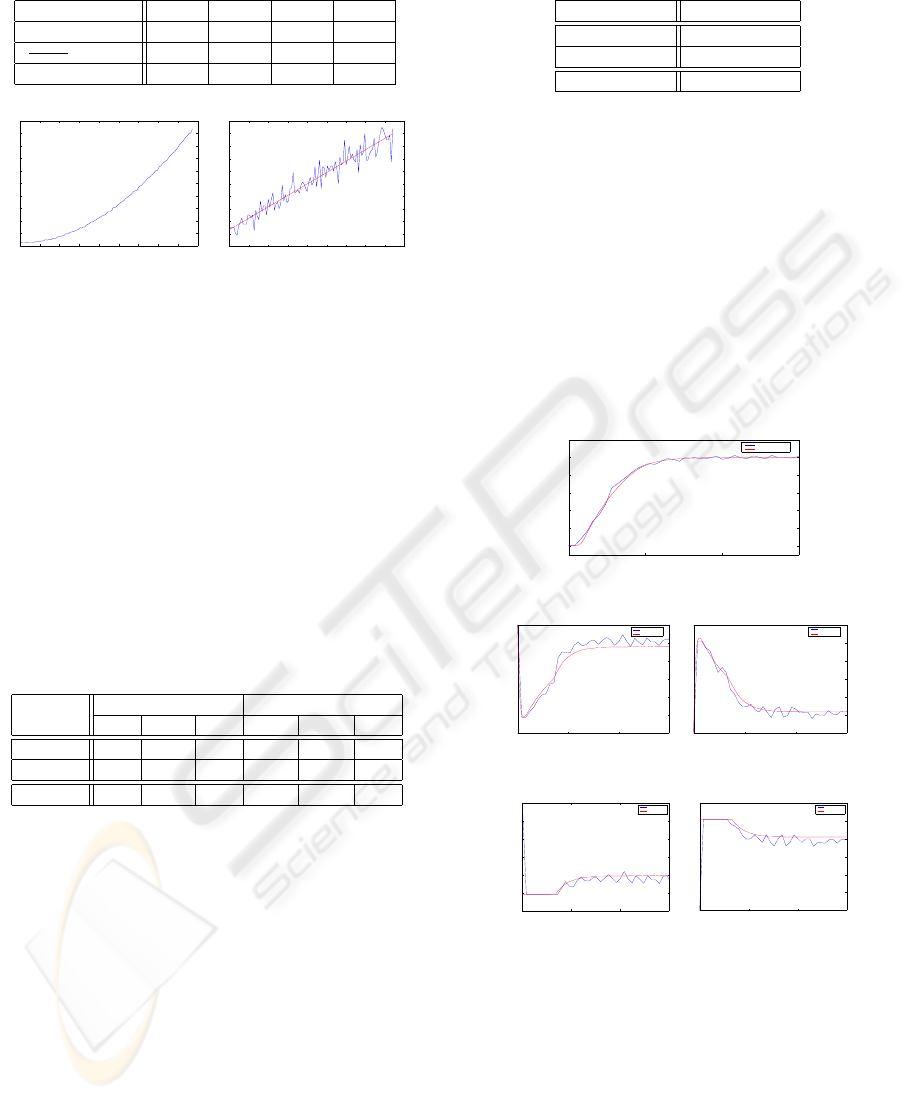
Table 4: Estimated inertia moments.

Exp. 1 Exp. 2 Exp. 3 Exp. 4

Γ(N.m) 1.2495 1.2495 1.2495 2.4500

dW (t)

(rad/s

)

0.9126 0.8942 0.8947 1.7512

J(kg.m

) 1.3691 1.3974 1.3965 1.3990

0 0.5 1 1.5 2 2.5 3 3.5 4 4.5

time[sec]

theta [rad]

(a) θ(t)(rad)

0 0.5 1 1.5 2 2.5 3 3.5 4 4.5

−0.5

0.5

1.5

2.5

3.5

4.5

time[sec]

W [rad/s]

(b) W(t)(rad/s)

Figure 9: First experiment.

3.4 Comparing Methods

The identiﬁed parameters are presented in tables 5

and 6. We can see a acceptable difference between

the estimated values, take into account that the exper-

iments had been made in hard conditions. For exam-

ple, the measured values of currents and velocities

have a considerable noise and any irregularity in the

ﬂoor can cause alterations in robot parameters. In the

model robot was used the mean of estimated parame-

ters.

Table 5: Estimated frictions.

Frictions Viscous Coulomb

Method 1 3.45 2.90 0.73 28.55 28.46 5.12

Method 2 4.01 3.77 - 30.35 30.76 -

Mean 3.73 3.34 0.73 29.45 29.61 5.12

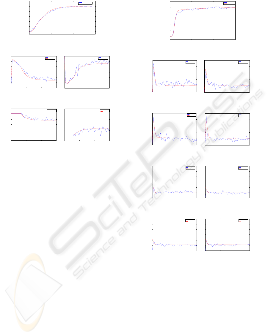
4 SIMULATION AND REAL

RESULTS

In this section the model simulation with the es-

timated parameters is presented. The simula-

tion environment was the Matlab/Simulink soft-

ware(Mathworks, 2000). Three simulations had been

made (see Figs.10, 11 and 12), using the following

reference velocities:

1. V = 1[m/s], V

= 0[m/s], W = 0[ rad/s];

2. V = 0[m/s], V

= 1[m/s], W = 0[ rad/s];

3. V = 0[m/s], V

= 0[m/s], W = 1[ rad/s].

The Figs. 10(a), 11(a) and 12(a) show the results of

the simulation and the real velocities of the robot. The

Table 6: Estimated inertia moments.

Inertia Moments

Methods 1+2 1.358

Method 3 (mean) 1.390

Mean 1.374

simulation results are very similar to the real ones, in

the transitory and the steady state too.

In Figs. 10(b), 10(c), 11(b) and 11(c) we can see

some non-linearities of the robot, due to PWM satu-

ration, shown in Figs. 10(d), 10(e), 11(d) and 11(e).

The simulated currents had a good approximation to

the real ones, because the model could ﬁnd even some

non-linearities of the system.

In third simulation(see Fig.12), the motors do not

saturate easily, because there are 4 motors simultane-

ously applying force. In this way, the transitory state

become much more fast.

0 0.5 1 1.5

0.2

0.4

0.6

0.8

Time[sec]

V[m/s]

Real

Simulated

(a) Real and simulated V (m/s).

0 0.5 1 1.5

−6

−5

−4

−3

−2

−1

Motor 2

Time[seg]

i2 [A]

Real

Simulated

(b) Current i2(A)

0 0.5 1 1.5

Motor 4

Time[sec]

i4 [A]

Real

Simulated

0 0.5 1 1.5

−300

−250

−200

−150

−100

−50

PWM motor 2

Time[seg]

Duty cycle[0..255]

Real

Simulado

(d) PWM motor 2

0 0.5 1 1.5

100

150

200

250

300

PWM motor 4

Time[sec]

Duty cycle[0..255]

Real

Simulado

(e) PWM motor 4

Figure 10: Velocity V = 1, simulation 1.

5 CONCLUSION

In this paper an experimental identiﬁcation of the dy-

namic parameters of an omni-directional mobile robot

has been developed. Three methods of the parameters

DYNAMIC PARAMETERS IDENTIFICATION OF AN OMNI-DIRECTIONAL MOBILE ROBOT

569

0 0.5 1 1.5

0.2

0.4

0.6

0.8

Vn[m/s]

Real

Simulated

Time[sec]

(a) Real and simulated V

(m/s).

0 0.5 1 1.5

Motor 1

Time[sec]

i1 [A]

Real

Simulated

(b) Current i1(A)

0 0.5 1 1.5

−6

−5

−4

−3

−2

−1

Motor 3

Time[sec]

i3 [A]

Real

Simulated

0 0.5 1 1.5

100

150

200

250

300

PWM motor 1

Time[sec]

Duty cycle[0..255]

Real

Simulado

(d) PWM motor 1

0 0.5 1 1.5

−300

−250

−200

−150

−100

−50

PWM motor 3

Time[sec]

Duty cycle[0..255]

Real

Simulado

(e) PWM motor 3

Figure 11: Velocity V

= 1, simulation 2.

identiﬁcation that even can be used in dynamic mo-

delling were described. A robot model that could ﬁnd

the non-linear elements is very important to design

of controllers and trajectories, mainly in application

where critical trajectories must be executed at higher

velocity, for example in robotic soccer. In the near fu-

ture, we will use the robot model to design controllers.

REFERENCES

Franklin, G. F., Powell, J., and Workman, M. (1997). Digi-

tal control of dynamic systems. Addison Weley Long-

man, Inc, 3 edition.

Liu, Y., Wu, X., Zhu, J. J., and Lew, J. (2003). Omni-

directional mobile robot controller design by trajec-

tory linearization. Proceedings of the American Con-

trol Conference, 4:3423 – 3428.

Mathworks, T. (2000). MATLAB Users’ Guide.

Watanabe, K. (1998). Control of ominidirectional mobile

robot. 2nd Int. Conf. on Knowledge-Based Intelligent

Electronic Systems.

0 0.5 1 1.5

0.2

0.4

0.6

0.8

Time[sec]

W[rad/s]

Real

Simulated

(a) Real and simulated W(rad/s).

0 0.5 1 1.5

0.5

1.5

2.5

Motor 1

Time[sec]

i1[A]

Real

Simulated

(b) Current i1(A)

0 0.5 1 1.5

0.5

1.5

2.5

Motor 3

Time[sec]

i3 [A]

Real

Simulated

0 0.5 1 1.5

0.5

1.5

2.5

Motor 2

Time[sec]

i2[A]

Real

Simulated

(d) Current i2(A)

0 0.5 1 1.5

0.5

1.5

2.5

Motor 4

Time[sec]

i4 [A]

Real

Simulated

(e) Current i4(A)

0 0.5 1 1.5

100

150

200

250

300

PWM motor 1

Time[sec]

Duty cycle[0..255]

Real

Simulated

(f) PWM motor 1

0 0.5 1 1.5

100

150

200

250

300

PWM motor 3

Time[sec]

Duty cycle[0..255]

Real

Simulated

(g) PWM motor 3

0 0.5 1 1.5

100

150

200

250

300

PWM motor 2

Time[seg]

Duty cycle[0..255]

Real

Simulated

(h) PWM motor 2

0 0.5 1 1.5

100

150

200

250

300

PWM motor 4

Time[sec]

Duty cycle[0..255]

Real

Simulated

(i) PWM motor 4

Figure 12: Velocity W = 1, simulation 3.

ICINCO 2006 - ROBOTICS AND AUTOMATION

570