A NEW METHOD FOR THE EVALUATION OF THE SIGNAL

ACQUIRED FROM QUANTITATIVE SEISMOCARDIOGRAPH

Hardware and Software Solution for the New Field of Monitoring Heart Activity

Z. Trefny, J. Svacinka, S. Trojan, J. Slavicek, P. Smrcka, K. Hana

Faculty of Biomedical Engineering, Czech Technical University in Prague, Studnickova 7, 2028 Prague 2, Czech Republic

Keywords: Time-domain segmentation of the seismocardiogram, J-wave recognition.

Abstract: The device for quantitative seismocardiography (QSCG) detects cardiac vibrations as they affect the entire

body; the measuring sensors (solid-state accelerometers) are usually placed in the plate of the chair –

additional instruments applied on the proband’s body are not required. The results of the QSCG analysis are

usable in various clinical fields. The first and most important step in the process of detection of significant

characteristics of measured QSCG curves is to detect pseudo-periods in the signal regardless of the initial

pseudo-period position. Other characteristics can be acquired by a relatively simple process over the

appointed pseudo-period. We have developed the experimental equipment for the QSCG measuring and

analysis. We have also developed special algorithms for preprocessing, segmentation and interactive

analysis of the QSCG signal. In this contribution we will introduce technical principles of the quantitative

seismocardiography and then we will focus on the original method for the basic segmentation of the QSCG

signal in time-domain; the method is easy, robust and is appropriate for real-time QSCG processing.

1 INTRODUCTION

Ballistocardiography (BCG): In 1936, Starr took

part in a conference held by the American Society of

Physiology which dealt with methods of determining

cardiac output. Thus began the era of high-

frequency ballistocardiography, which lasted

approximately 15 years. Other types of instruments

were developed, on which the displacement, velocity

or acceleration of a body lying on a bed was

measured. Later studies showed that there are

difficulties when comparing records registered on

different apparatuses. This is mainly caused by two

factors: (a) the instrument’s natural frequency, (b)

the instrument’s damping.

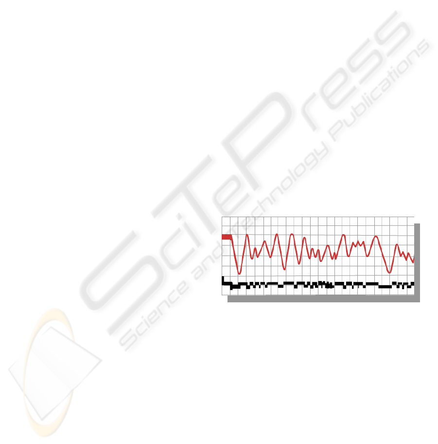
Figure. 1: Records registered using the old BCG

instrument with a frequency of 2Hz and critical damping.

The lower curve depicts the effect of force applied, which

is still of the same intensity but differs in the duration of

its effect. The upper curve is a record, from which one

cannot determine either size or duration of the acting

force.

Quantitative ballistocardiography (QBCG):

Following the critical evaluation of all these facts,

we began in 1952 our own experiments related to the

construction of an apparatus which would lack the

aforementioned shortcomings. Thus, over the years,

we constructed an apparatus whose advantages lie

not only in the simplicity of its design, but also in its

important functional qualities. To achieve a minimal

distortion caused by the transmission from the origin

Trefny Z., Svacinka J., Trojan S., Slavicek J., Smrcka P. and Hana K. (2006).

A NEW METHOD FOR THE EVALUATION OF THE SIGNAL ACQUIRED FROM QUANTITATIVE SEISMOCARDIOGRAPH - Hardware and Software

Solution for the New Field of Monitoring Heart Activity.

In Proceedings of the Third International Conference on Informatics in Control, Automation and Robotics, pages 61-66

DOI: 10.5220/0001220000610066

 SciTePress

of the force to the recorder it is necessary that the

natural frequencies of the transmission systems lie as

far as possible from the mentioned frequency range.

The cardiovascular activity is manifested by a

force acting on the human body which represents a

mechanical vibratory system transmitting the force

to the balistocardiographic apparatus.

The basic part of our portable quantitative

balistocardiograph is a very rigid piezoelectric force

transducer resting on a rigid steel chair. The

examined person sits (Figure 2) on the light seat

placed on the transducer and the force caused by the

cardiovascular activity is measured in this way. The

output of the piezoelectric pick-up is fed into an

operational amplifier.

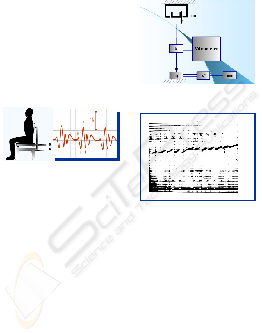
Figure 2: Position of the examined person during the

QBCG session.

The advantage of the piezoelectric transducer is

in very low compliance together with a very high

natural frequency of the apparatus. Another

advantage of the rigid pick-up is the fact that it can

be preloaded with a substantial static force – the

weight of the examined person, and it is still

possible to measure the alternating forces of the

magnitude of g+ (gram as weight). The simple push

button is used to dispose of the static charge caused

by the weight of the person. The measured force is

registered (REG).

Dynamic calibration of the QBCG apparatus was

carried out by an electrodynamic exciter (EXC)

acting via a calibrated dynamometer (D), also of a

piezoelectric type, on a pick-up (Q) of the QBCG

(see Figure 3).

Figure 3: A set-up a dynamic calibration of the

quantitative balistocardiographic apparatus.

Figure 4: Records registered using the QBCG instrument.

The lower curve depicts the effect of force applied. The

upper curve is a record, from which we can determine size

and duration of the acting force. Compare with BCG

record on Figure 1.

Quantitative seismocardiography: (QSCG: This

method enables the recording of force applied

without phase or time deformation. Thus, heart rate

may be monitored and analysed using the method of

heart rate variability (statistical and autocorrelation

analysis, spectral analysis, total effect of regulation,

vegetative homeostasis, activity of subcortical

centre, activity of the vasomotor centre and stress

index). The method of QSCG was designated by the

laboratory employees as an absolutely non-invasive,

and the persons examined did not have any

electrodes attached to the body surface and were not

connected by cables to the registering instrument.

This new field of monitoring heart activity, whereby

we determine both amplitude-force and time-

frequency relationships, is termed quantitative

seismocardiography. Thus, one may determine the

force-response of the cardiovascular system to

ICINCO 2006 - SIGNAL PROCESSING, SYSTEMS MODELING AND CONTROL

changes in external stimuli, as well as the

autonomous nervous system regulation of the

circulation and the activity of the sympathetic and

parasympathetic systems.

2 METHODS OF QSCG

MEASUREMENT AND

ANALYSIS

2.1 Experimental Equipment

In terms of practical use, a portable telemetric

system for the QSCG measuring has been

developed. This system allows data to be acquired

and assessed using quantitative seismocardiography

(QSCG) and triaxial accelerometric measurements

on the thorax of a patient. It is composed of the three

HW modules that are telemetrically interconnected

with the option of interconnecting through a metallic

line. These are the seismocardiographic, the

accelerometric modules and a module for the data

transfer interconnected with the PC through the USB

interface. Block scheme of the whole system is on

figure 7.

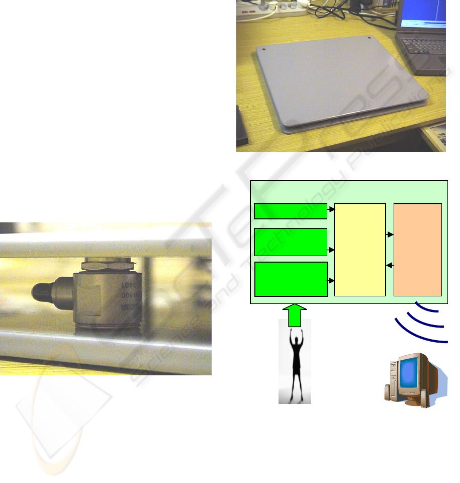
Figure 5: Main sensor of she QSCG measuring equipment

- detail of the solid-state accelerometer between measuring

metal plates.

Sensing mechanical body reactions, which are

induced in response to the cardiovascular dynamics,

is provided by the seismocardiographic module,

which reads the strain coming from the mechanical

deformation of the piezo-electric plate. This sensing

module is mounted on a special device, which works

by transmitting the mechanical body reactions onto

the piezo-electric recorder. The accelerometric

module is applied for measuring thorax acceleration

as induced by movements from the heart activity,

this measurement is made on the three basic

orthogonal axes. The core of the module is the

sensing device composed of the two biaxial

monolithic semiconductor accelerometers. The data

transfer module is designed to transmit the data from

the radio-module into the PC through the USB

interface.

Figure 6: Measuring plates of the proposed QSCG device.

Figure 7: Block scheme of the experimental QSCG device.

2.2 Algorithm for the Time-Domain

Segmentation of the QSCG

We have developed algorithms for preprocessing,

segmentation and interactive analysis of the QSCG

signal. In this contribution we will focuse on the

original method for basic segmentation of the QSCG

Control

unit,

A/D

Converter

Commu-

nication

interface

WIFI

Bluetooth

SCG unit

ECG measuring

unit

Auxiliary

measuring units

PATIENT‘S MEASURING DEVICE

PATIENT

WORKSTATION

FOR

SUPERVISON,

DATA

PROCESSING

WIRELESS CONNECTION

A NEW METHOD FOR THE EVALUATION OF THE SIGNAL ACQUIRED FROM QUANTITATIVE

SEISMOCARDIOGRAPH - Hardware and Software Solution for the new Field of Monitoring Heart Activity

signal in time-domain; this first step is crucial for the

successfulness of the whole diagnostic process. Our

method is relatively simple and was developed for

the detection of QSCG pseudo-periods in real time.

The method is derived from a well-known and

robust algorithm for QRS complex detection in

traditional electrocardiograms (ECG), originally

developed by Hamilton et al. The algorithm was

based on the first derivative of the input signal and

many thresholds and parameters are automatically

adapted to individual changes in the input signal

using sophisticated empirical rules. The results

(position of the dominant – so-called R - wave) are

obtained with some detection delay (above 200 ms).

For details on the algorithm, see [Hamilton].

For our purposes it is important that the initial

values of many parameters are adjustable and by

modification of these values the original method was

slightly adapted to QSCG’s different curve

morphology. Namely the following parameters were

changed: (1) length of the first derivative from the

original 10 ms to 80 ms, (2) length of the high-pass

pre-filter from 125 ms to 350 ms, (3) length of

moving window integration from 80 ms to 200 ms.

Optimal values were selected experimentally in

order to achieve the best detection results.

Additionally, we developed a special backward

searching process for the precise detection of the

position of the I-wave and J-wave in each QSCG

pseudo-period.

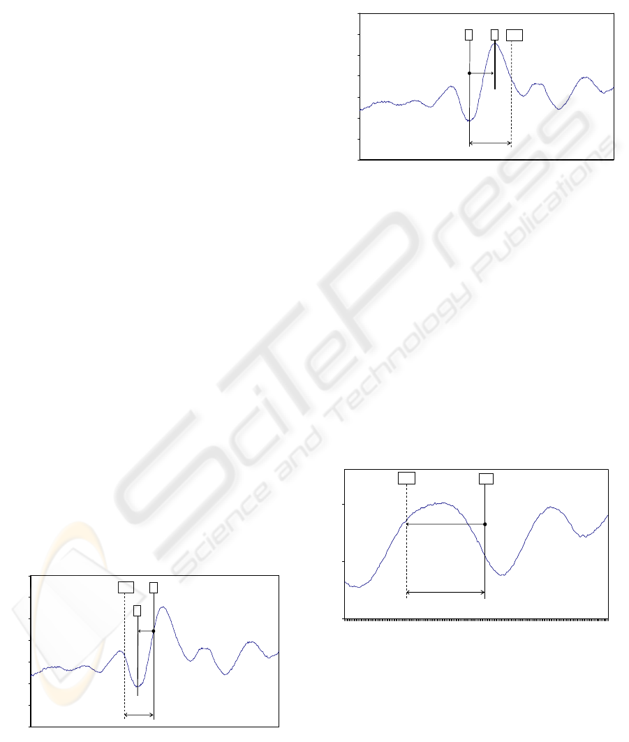
The function of the whole algorithm is as follows:

output of the traditional ECG QRS detector gives the

rough position of the systolic complex inside the

QSCG - candidate X. Then the specific morphology

of the QSCG curve is utilized to backward search

the position of the J-wave – we expect the first big

negative peak in MTI samples (about 100 ms). If the

detection is successful, we assign the position of the

peak as the I-wave; see Figure 8.

6000

7000

8000

9000

10000

11000

12000

13000

1 58 115 172 229 286 343 400 457

time [samples]

Force (quant. le ve ls )

max

MTI

Figure 8: Backward local I-peak searching in the QSCG

cycle.

Finally we search forward for the position of the

J-wave, which we expect to be the first big positive

peak in maximally MTJ samples (about 160 ms), see

Figure 9.

6000

7000

8000

9000

10000

11000

12000

13000

1 58 115 172 229 286 343 400 457

time [samples]

Force (quant. le ve ls )

I J

max

MTJ

Figure 9: Forward local J-peak searching in the QSCG

cycle.

For the peak-detection we used a very simple

method based on the first difference (length 15 ms):

when the transition from negative to positive value

of the difference occurs, then the sequence is marked

as a negative peak; the transition from a positive to

negative difference means a positive peak. If

searching for the J-wave or the I-wave fails,

candidate “X” is rejected and the algorithm

continues without detection of the QSCG pseudo-

period.

The rejection of “candidate X” is very important

step and it increases robustness of the whole

detection procedure against the artifacts – see

demonstration on the Figure 10.

8800

10800

12800

1 11 21 31 41 51 61 71 81 91 101 111 121 131 141 151 161 171 181 191 201 211 221

time (samples)

Force (quant. levels)

max

MTI

Figure 10: Rejection of the false beat detection. We search

backward from “candidate X3” for the first big negative

peak. The I-wave must be recognized in MTI samples

(about 100 ms), so in this case the detection was not

successful.

The false detection of the dominant “candidate

X”, which is not a true QSCG cycle, was corrected

by the proposed simple backward searching

ICINCO 2006 - SIGNAL PROCESSING, SYSTEMS MODELING AND CONTROL

algorithm, because the morphology in the nearest

neighborhood of the point X3 does not match the

detection rules – backward searching for the I-wave

in MTI samples was not successful, the false

positive detection of the systolic complex was

correctly rejected.

5000

7000

9000

11000

13000

15000

1 73 145 217 289 361 433 505 577 649 721 793 865 937 1009 1081 1153 1225

time (samples)

Force (quant. levels)

X2 X3 X4

Figure 11: Result of the whole detection: false candidate

X3 was correctly rejected.

The whole software system contains additional

modules for statistical and autocorrelation analysis,

spectral analysis, assessment of the aggregated effect

of the regulation of autonomous functions of

vegetative homeostasis, activity of the vasomotor

centre, activities of the sympathetic cardiovascular

centre and the stress index (SI). Our experimental

software allows also automatic extraction of

classical QSCG hemodynamical parameters,

especially so called systolic force (SF). The current

version of the system is designed for OS Windows

XP and has user-friendly interface. Block scheme of

the system is on figure 12:

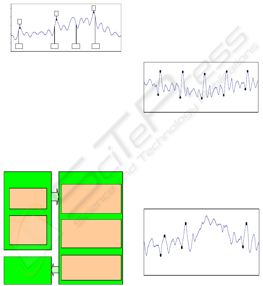
Figure 12: Block scheme of the software system.

Presented algorithm is in the box „Unit for time-domain

segmentation of the QSCG curves“.

3 CONCLUSION

For high-quality measurements we can obtain good-

looking signals for which both methods exhibit

excellent results. For disruptive and spurious signals

there is still a good chance of obtaining authentic

information because we first detect the impairments

and remove the particular interval of the signal. It is

true that in using this method we also remove certain

useful information but simultaneously ensure

processing of the remaining signal. We emphasize

that we need not process all consecutive pseudo-

periods in the signal but only a sufficient amount of

pseudo-periods.

4000

6000

8000

10000

12000

14000

1 70 139 208 277 346 415 484 553 622 691 760 829 898 967 1036 1105 1174 1243 1312 1381 1450

Force (quant. levels)

time (samples)

J J

Figure 13: Typical QSCG signal with correctly placed

reference points.

For good-looking and typical signals, the

methods behave very well, achieving nearly

complete success (see Figure 13). The success

decreases with deterioration of the signal. On the

other way, in such signals it is often difficult even

for the human expert to recognize correct pseudo-

period time points (see Figure 14).

2000

4000

6000

8000

10000

12000

14000

16000

18000

1 70 139 208 277 346 415 484 553 622 691 760 829 898 967 1036 1105 1174 1243 1312 1381 1450

Force (quant. levels)

time (samples)

I I

J J

Figure 14: QSCG signal with the motion artifact; it is

difficult to recognize correct positions of some reference

points.

Measuring

software

Visualization,

printing and

archivation

Setup and

calibration

Signal

acquisition

and data

storage

Data processing uni

Unit fo

time-domain

segmentation of the

QSCG curves

Unit for extraction of

the

hemodynamical

parameters

Unit for extraction of

the HRV parameters

A NEW METHOD FOR THE EVALUATION OF THE SIGNAL ACQUIRED FROM QUANTITATIVE

SEISMOCARDIOGRAPH - Hardware and Software Solution for the new Field of Monitoring Heart Activity

The QSCG signal offers specific information

about functional changes of the cardiovascular

system regulation which preceded the structural

changes coming later. The equipment is ready for

use, algorithms for automatic analysis of the QSCG

signal are prepared.

Quantitative seismocardiography probably offers

a more complex view of both inotropic and

chronotropic heart function. It will be suitable for:

examining operators exposed to stress; for assessing

the effect of work, fatigue, mental stress; for

monitoring persons as part of disease prevention; for

determining a person’s ability to carry out their

duties both on the ground and in the air.

ACKNOWLEDGEMENTS

This work has been supported by the Ministry of

Education of the Czech Republic under project No.

MSM6840770012 and by the project UREKA

E!3031.

REFERENCES

Jerosch-Herold, M. et al., 1999. The seismocardiogram as

magnetic-field-compatible alternative to the

electrocardiogram for cardiac stress monitoring, In

International Journal of Cardiac Imaging, 15(6), pp.

523-31

Trefny, Z. et al., 1996: Some physical aspects in

cardiovascular dynamics, In J. Cardiovasc. Diagnosis

and Procedures, 13(2), pp. 141 - 145

Hamilton, P. – Tompkins, W.J. (1987): Quantitative

investigation of QRS detection rules using the

MIT/BIH arrhythmia database, In IEEE Trans.

Biomed.Eng., 33, pp. 1158-65

Trefny Z. – David E. - Bayevsky R.M.: Achievements in

Space Medicine into Healt Care Practice and Industry,

Development of Space Cardiology metods in the

Earth's Health Service, Berlin 2001

Freisen G., Jannet T.: A comparison of the Noise

Sensitivity of Nine QRS Detection Algorithms’, IEEE

Trans. Biomed. Eng., 1990, 85(1)

ICINCO 2006 - SIGNAL PROCESSING, SYSTEMS MODELING AND CONTROL