
ESTIMATION OF PERFORMANCE OF HEAVY VEHICLES BY
SLIDING MODES OBSERVERS
N. K. M’Sirdi, A. Boubezoul, A. Rabhi
LSIS, CNRS UMR6168
Dom. Univ. St Jrme, Av Escadrille Normandie-Niemen 13397 Marseille, France
L. Fridman
UNAM Dept of Control, Div. Electrical Engineering
Faculty of Engineering, Ciudad Universitaria, Universidad Nacional Autonoma de Mexico, 04510, Mexico, D.F., Mexico
Keywords:
Heavy Vehicle Modeling, Sliding Mode Observers, First and second order sliding modes, Estimation of inputs.
Abstract:
The objective of this work, is performance handling and maneuverability, by means of the observation of
vehicle dynamics in order to obtain safer and an easier driving. First and second order sliding mode observers
are developed to estimate the vehicle state. Lateral forces are estimated in a last step.
1 INTRODUCTION
The work of this paper has been done in context of
the national French project ARCOS 2004. The main
objective is to develop predictive procedures allowing
to detect risky situations and produce alarms.
Heavy lorries are population of risky vehicles, both
for themselves and other vehicles. It is known that
risk of having dead people accidents involving trucks
is multiplied by 2,4 in comparison to the same risk for
accident involving only light vehicles.
The study of a 581 accidents lorries sample involv-
ing 616 trucks gave the following statistics recorded
in an accident database owned by Renault Trucks and
CEESAR (Desfontaines, 2004). Accidents involv-
ing heavy lorries have serious consequences for road
users, and incidents induce major congestions or dam-
age to the environment or the infrastructure at a dis-
proportionate economic cost. A large number of car
accidents is attributed by statistic studies to increase
of presence of heavy vehicles. For the accidents in-
volving at least one truck, the truck is alone in 33 %
of the cases. These accidents are of three types : 20
% rollover, 11 % the road departure and 2 % jack-
knifing. The truck structure often concerned by these
accidents is a tractor and the semi trailer. This type of
truck is involved for: 45 % in the whole database, and
80 % of those involved in a rollover (Desfontaines,
2004).
0
ARCOS 2004 is supported by CNRS, ministry of
research and education and ministry of equipment of the
French government.
To improve safety, several solutions have been
studied in programs on Intelligent Transporta-
tion Systems (US NAHSC Program, California
PATH Program, Japan’s AHSRA, European Pro-
grams: ADASE, REPONSE and CHAUFEUR-
driven, French PREDIT and ARCOS Programs, etc.).
Some orientations of these programs are control help
for drivers and active safety systems, fully automated
operation, detection and warning messages when un-
der dangerous conditions... In literature, several pro-
cedures have been proposed to detect instabilities in
the vehicle dynamics (Dahlberg, 2001) (R. Ervin,
1998) (P. J. Liu, 1997) (S. Rakheja, 1990). In general
lateral slips, over steering or roll over situations are
detected by processing measurements. The main in-
formation needed to prevent risky situations, are the
vehicle states and input contact forces. This knowl-
edge is necessary for forward prediction of behavior
and preview control or safe monitoring.
In this paper, we focus our work to on-line esti-
mation of tires forces in a cornering manoeuver at
constant speed. The organization is as follows. Sec-
tion 2 develops a simplified model. Two observers
are designed in section 3. The first one is based on
first order sliding mode and backstepping to estimate
the system state and then we deduce the applied tire
forces. The second observer uses the super twist-
ing algorithm (second-order sliding mode) to observe
states and then identify or estimate the tires forces.
The section 4 will discuss the simulation results and
validation. A conclusion is given to emphasize in-
terest of these results for predictive diagnosis giving
embedded help systems for safe driving.
360
M’Sirdi N., Boubezoul A., Rabhi A. and Fridman L. (2006).
ESTIMATION OF PERFORMANCE OF HEAVY VEHICLES BY SLIDING MODES OBSERVERS.
In Proceedings of the Third International Conference on Informatics in Control, Automation and Robotics, pages 360-365
DOI: 10.5220/0001219903600365
Copyright
c
SciTePress
2 HEAVY VEHICLES NOMINAL
MODEL
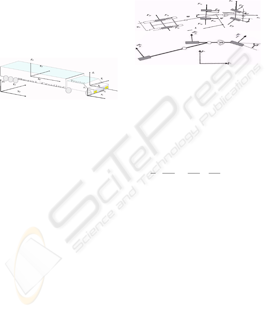
2.1 Vehicle Description
The vehicle considered in this work is a tractor-semi-
trailer with 5-axels (figure 1). To estimate the dy-
namics in a cornering manoeuver, we adopt a simple
configuration to describe our heavy vehicle (C.Chen,
1997). The tractor has a body with 2-axels and the at-
tached semi-trailer is made of a body supported by 3
axels. To deduce the model, we consider the follow-
Figure 1: Tractor and semi-trailer vehicle (components);
The System Coordinates and reference frames.
ing assumptions for simplification.
·The pitch and bounce dynamics are neglected,
tractor and trailer have rigid bodies. Only dynamics of
two bodies (i.e. tractor and trailer’s) are considered.
·The total suspension motions are reduced to the
roll of suspension axels only.
·The essential dynamics considered here are the
yaw and horizontal translation motions, the tractor
roll angle and articulation angle between the tractor
and trailer (see figure 2). The trailer’s roll angle is
measured around the tractor roll axis.
The dynamics equations of the motion of the two
sprung masses is written in a coordinate reference
frame R
E
(X
E
Y
E
Z
E
) attached to the earth (see figure
1). The frames R
T
(X
t
Y
t
Z
t
) and R
ST
(X
st
Y
st
Z
st
)
are attached to the gravity centers of the trac-
tor and semi-trailer’s sprung masses (respectively).
(X
u
Y
u
Z
u
) is the frame of tractor’s unsprung mass
(fixed at center of the front axle with Z
u
is parallel
to Z
E
, see figure 2).
The relative motion of X
u
Y
u
Z
u
with respect to
the earth-fixed coordinate system X
E
Y
E
Z
E
describe
the translation motion of the tractor in the horizon-
tal plane and its yaw motion along Z
E
axis. The roll
motion is described by motion of coordinate X
t
Y
t
Z
t
relative to the coordinate X
u
Y
u
Z
u
. The articulation
angle between the tractor and trailer can be described
by relative motion of the coordinate X
t
Y
t
Z
t
with re-
spect to the coordinate X
t
Y
t
Z
t
.
With this coordinate systems and description of
their relative motion, we consider the following gen-
eralized coordinates:
x
E
: position of the tractor gravity center in R
E
,
y
E
: position of the tractor gravity center in R
E
,
ψ : yaw angle of the tractor,
φ : roll angle,
ψ
f
: angle between tractor and trailer (relative
pitch).
Figure 2: a: Applied forces on the tractor and semi trailer
vehicle. The Motions of the system parts. b: The extended
Bicycle Model.
2.2 Dynamic Model
The previous description of the vehicle motion allows
the calculation of the translational and rotational ve-
locities of each body-mass at C.G. and kinematics
with respect to different references frames. The total
kinetic energy (E
K
) and potential energy (E
P
) are ex-
pressed in the frame R
E
(X
E
Y
E
Z
E
). The Lagrange
approach leads to the following vehicle model:
d
dt
∂E
K
∂ ˙q
i
−
∂E
K
∂q
i
+
∂E
P
∂q
i
= F
g
i
M(q)¨q + C(q, ˙q) ˙q + G(q) = F
g
(1)
where q
i
is the i
th
generalized coordinate and q is
the generalized coordinate vector defined as q =
[x, y, ψ, φ, ψ
f
]. The matrix M (q) represent the sym-
metric and positive definite inertia matrix. The vector
C(q, ˙q) ˙q gives the Coriolis and Centrifugal forces and
G(q) is the gravity force vector. The effects of the last
tree axels are regrouped in one equivalent.
As generalized forces, the vector F
g
represents the
wheels - road contact forces acting on the system bod-
ies. This vector is made of vertical, longitudinal and
lateral forces due to contact between the wheels and
the road (see figure 2) (Pacejka and Besselink, 1997).
To link these tires forces and their effects on bodies
motion, an extended bicycle model is used (Acker-
mann, 1998)(N.K. M’sirdi and Delanne, 2004). The
locations of these external forces are considered at
each wheel of the three axles.
The tire-road interface forces F
g
are related to the
suspensions of each wheel through the three axles.
Suspensions are modeled as a combination of a spring
and a damper elements. Owing to robustness of Slid-
ing Mode approach, with respect to the modeling er-
rors (?)(Utkin, 1977)(Slotine et al., 1986), we use
ESTIMATION OF PERFORMANCE OF HEAVY VEHICLES BY SLIDING MODES OBSERVERS
361

only a simple linear nominal model for suspension.
F
sf
i
= F
0f
i
+ K
f
z
f
i
+ D
f
˙z
f
i
F
sr
i
= F
0r
i
+ K
r
z
r
i
+ D
r
˙z
r
i
F
st
i
= F
0t
i
+ K
t
z
t
i
+ D
t
˙z
t
i
for i = 1, 2
(2)
where F
0
i
is the static equilibrium force and z
i
de-
fine the deflection of the spring from its equilibrium
position with K and D the suspension parameters.
For nominal model, as we consider that the suspen-
sion forces are due only to rolling motion, the deflec-
tion variables z
i
are given as:
z
f
1
= −z
f
2
= −
w
f
2
sin(φ)
z
r
1
= −z
r
2
= −
w
r
2
sin(φ)
z
t
1
= −
w
t
2
sin(φ) cos(ψ
r
) + l
t
φ sin(ψ
r
)
z
t
2
=
w
t
2
sin(φ) cos(ψ
r
) + l
t
φ sin(ψ
r
)
(3)
To include tire forces in the model, we consider
a cornering manoeuvre realized at constant speed.
Then, the longitudinal forces are assumed nulls. The
total tire/road adhesion is considered toward the lat-
eral direction (figure 2). In this model, the unknown
inputs are the lateral tire forces at the front and rear
axles of the tractor and the one at the semitrailer
equivalent (rear) axle. These forces will be repre-
sented by the vector F = (F
f
, F
r
, F
t
).
The vehicle model (1), developed in the inertial
frame, depends on the position and orientation of the
vehicle in this reference. However, the measurements
used generally in vehicles to analyze the dynamics are
defined in the vehicle unsprung mass frame. Then,
we will rewrite the vehicle model (1) (inertial refer-
ence) with respect to this reference frame (unsprung
mass reference frame) using the transformation ma-
trices between those coordinates. Then we obtain
˙x
E
cos(ψ) + ˙y
E
sin(ψ) = v
x
− ˙x
E
sin(ψ) + ˙y
E
cos(ψ) = v
y
¨x
E
cos(ψ) + ¨y
E
sin(ψ) = ˙v
x
− v
y
˙
ψ
−¨x
E
sin(ψ) + ¨y
E
cos(ψ) = ˙v
y
− v
x
˙
ψ
(4)
where ˙x
E
and ˙y
E
are respectively the vehicle veloc-
ities in the inertial reference frame. v
x
and v
y
are
respectively the vehicle velocity components along
the axes X
u
and Y
u
in the unsprung mass reference
frame. The transformation of the generalized forces
is obtained in the same way:
F
x
= F
g
x
cos(ψ) + F
g
y
sin(ψ)
F
y
= −F
g
x
sin(ψ) + F
g
y
cos(ψ)
(5)
where F
x
and F
y
are the external forces respectively
along the X
u
and Y
u
. They are expressed in function
of lateral tire contact forces, steering angle δ and ar-
ticulation angle ψ
f
.
3 OBSERVERS DESIGN
To estimate lateral forces, we propose in this section
to develop an observer based on the first order sliding
mode approach followed by an estimator.
3.1 Model Parametrization
The state variables of the model expressed in the un-
sprung mass reference frame are as follows:
˙x = f (x, δ, F ) (6)
x = (φ, ψ
f
, v
x
, v
y
,
˙
ψ,
˙
φ,
˙
ψ
f
) (7)
with
˙
ψ,
˙
φ,
˙
ψ
f
to represent respectively the yaw, the
roll and the rate of change of the articulation angle
ψ
f
. Here F represent the unknown input forces and
the steering angle δ represent the known system input
(M’sirdi et al., 2006).
In our case, we assume available for measurements
the roll angle φ, the angle between tractor and trailer
(relative yaw at the fifth wheel) ψ
f
, the yaw velocity
˙
ψ and the vehicle velocities v
x
and v
y
. The unknown
variables are the state components
˙
φ and
˙
ψ
f
, and lat-
eral tire forces F . The state vector is then split in two
parts x
T
= [x
T
1
, x
T
2
]
T
with: x
1
= (φ, ψ
f
)
T
measured
and x
2
=
v
x
, v
y
,
˙
ψ,
˙
φ,
˙
ψ
f
T
.
The system (6) can then be written
(
˙x
1
= ρ x
2
˙x
2
= f
1
(x
1
, x
2
) + f
2
(x
1
, δ, F )
y = x
1
(8)
where ρ =
0 0 0 1 0
0 0 0 0 1
, and f
1
et f
2
are
analytic functions defined in <
5
.
The function f
1
(x
1
, x
2
) may be parameterized as:
f
1
(x
1
, x
2
) = ϕ (x
1
, x
2
, δ) .θ
o
+ ζ with θ
o
a vector of
nominal system parameters (θ
o
the nominal values of
the vector θ) and, ϕ (x
1
, x
2
, δ) a regression vector de-
pending on well-known functions of (x
1
, x
2
, δ). The
remaining term ζ is a small and bounded perturbation
representing modeling errors due to use of approxi-
mations. The function f
2
(x
1
, δ, F ) may be written
f
2
(x
1
, δ, F ) = Ω (x
1
, δ) F (9)
f
1
(x
1
, x
2
) = ϕ (x
1
, x
2
, δ) .θ
o
+ ζ (10)
Ω is a matrix in <
3x5
. The vector x
2
is composed of
both measured variables v
x
, v
y
and
˙
ψ, and unknown
variables
˙
φ,
˙
ψ
f
. The vector x
2
= (x
21
, x
22
)
T
is made
of two components, the first part x
21
= (v
x
, v
y
,
˙
ψ)
T
is measured and x
22
= (
˙
φ,
˙
ψ
f
)
T
the unknown vari-
ables to be robustly observed.
The model may be rewritten in an explicit triangu-
lar form with Bounded Input and finite time Bounded
State (BIBS) a follows(M’Sirdi et al., 2000)
˙x
1
= ρx
2
= x
22
˙x
2
= D
x
21
x
22
+ Ω (x
1
, δ, F )
y = x
1
(11)
ICINCO 2006 - ROBOTICS AND AUTOMATION
362

The matrix D defined in R
5×5
depends on the state
x and Ω is a matrix defined in R
5×3
.
3.2 First Order SM Observer
3.2.1 The Backstepping Observer
To estimate both forces and velocities, starting with as
measurement x
1
and x
21
, we propose the following
sliding mode observer giving the estimates ˆx
1
, ˆx
22
in
two steps(M’Sirdi et al., 2000)(N.K. M’sirdi and De-
lanne, 2004):
˙
ˆx
1
= ˆx
22
+ Λ
1
Sign
1
(x
1
− ˆx
1
)
˙
ˆx
2
= D
x
21
¯x
22
+ Ω (x
1
, δ)
ˆ
F + η
(12)
η =
Λ
21
0
0 Λ
22
Sign
2
(x
21
− ˆx
21
)
Sign
2
(¯x
22
− ˆx
22
)
(13)
Λ
1
, Λ
21
, Λ
22
are observer gains to be adjusted for
convergence,
ˆ
F is an a priori estimation of the forces
and Sign
i
is the vector of sign functions for t > t
1
.
The auxiliary variable ¯x
22
is introduced to design a
backstepping triangular observer (see (M’Sirdi et al.,
2000) for this observer):
¯x
22
= ˆx
22
+ Λ
1
Sign
1,moy
(x
1
− ˆx
1
) (14)
3.2.2 Finite Time Convergence of the Observer
For the convergence analysis, we express the state es-
timation error (˜x
i
= ˆx
i
− x
i
) dynamics equation.
Owing to the system triangularity we can study its be-
havior step by step.
˙
˜x
1
= ˜x
22
− Λ
1
Sign
1
(x
1
− ˆx
1
)
˙
˜x
2
= ∆ + Ω (x
1
, δ)
˜
F − η
(15)
∆ = D
x
21
x
22
−
ˆ
D
x
21
¯x
22
(16)
˜
F = F −
ˆ
F (17)
Step 1: Finite time convergence of ˆx
1
tox
1
in t
1
:
During this step the second sign is chosen null
Sign
2
∼
=
0 for t < t
1
. The observation error dynamic
(15) becomes:
˙
˜x
1
= ˜x
22
− Λ
1
Sign
1
(x
1
− ˆx
1
)
˙
˜x
21
˙
˜x
22
= ∆ + Ω (x
1
, δ)
˜
F (18)
Let us recall that the system is BIBS and consider
the following Lyapunov candidate function and com-
pute its derivative
V
1
=
˜x
T
1
˜x
1
2
(19)
˙
V
1
= ˜x
T
1
(˜x
22
− Λ
1
Sign (˜x
1
)) (20)
If we chose Λ
1
= diag (λ
1
, λ
2
) such as λ
i
>
k ˜x
22
(i) k
max
for any i = 1, 2, then
˙
V
1
< 0 and con-
sequently the observation error ˜x
1
goes to zero in a fi-
nite time t
1
. After t
1
is reached we have
˙
˜x
1
= 0. Then
after the Fillipov solution (Fillipov, 1960), we obtain
in the mean average ˜x
22
(i) = λ
i
Sign
eq
(˜x
1
(i)).
Owing to that Sign
eq
∼
=
Sign
m
on the sliding sur-
face (˜x
1
= 0), we deduce that ¯x
22
(i) = x
22
(i) and
then ¯x
22
= x
22
. Note that Sign
m
is the mean of
Sign, this can be considered as a low pass filtering
used to reduce the chattering effect in sliding modes
of the first order.
Step 2 : In this step, we are interested by conver-
gence of ¯x
22
in a finite time t
2
. Thereafter the es-
timation of the unknown input F can be processed.
Let us first replace the vector Sign
2
by the usual sign
functions (t > t
1
)
˙
˜x
1
= 0 = ˜x
22
− Λ
1
Sign
1
(˜x
1
)
˙
˜x
2
= ∆+Ω (x
1
, δ)
˜
F − Λ
2
Sign (˜x
2
)
The second Lyapunov function considered is:
V
2
=
˜x
T
1
˜x
1
2
+
˜x
T
2
˜x
2
2
(21)
˙
V
2
= ˜x
T
2
˙
˜x
2
for t > t
1
(22)
˙
V
2
= ˜x
T
2
∆ + Ω (x
1
, δ)
˜
F − Λ
2
Sign (˜x
2
) (23)
Knowing that
˜
F is bounded and choosing
λ
2
= diag (γ
1
...γ
5
) with γ
i
large enough (γ
i
>
|∆ + Ω (x
1
, δ)|
max
), the convergence of ˜x
2
to zero
is guaranteed in a finite time t
2
> t
1
then we will
have
˙
˜x
2
= 0, consequently. Then we obtain:
∆+Ω (x
1
, δ)
˜
F − Λ
2
Sign
eq
(˜x
2
) = 0 (24)
3.2.3 Unknown Input Estimation
As ¯x
22
= x
22
, then as we have chosen
ˆ
D ≈ D and
then ∆ ≈ 0. Let us define Q = Ω
T
Ω and assume that
it is invertible. The observation error dynamic is then:
˜
F = Q
−1
Ω
T
Λ
2
Sign
eq
(˜x
2
) = F −
ˆ
F (25)
Now, we can define a vector
¯
F as being an estimation
of forces. Furthemore, after the first and second step
(for t > t
2
) as we have ¯x
2
= x
2
, the expression of
this vector
¯
F becomes:
¯
F =
ˆ
F + Q
−1
Ω
T
Λ
2
Sign
m
(˜x
2
) (26)
¯
F =
ˆ
F + Q
−1
Ω
T
Λ
Sign
2,moy
(x
21
− ˆx
21
)
Sign
2,moy
(¯x
22
− ˆx
22
)
After time reaches t
2
we have Sign
eq
(.)
∼
=
Sign
m
(.), during this second step the signal ¯x
2
= x
2
is reached, assuming that conditions of the first step
ESTIMATION OF PERFORMANCE OF HEAVY VEHICLES BY SLIDING MODES OBSERVERS
363

remain valid after t
1
, we can then conclude that for
any t > t
2
we have
¯
F ' F in the mean average.
Then the observer proposed (equations (12) and
(14)) with respect to depicted conditions and the gain
matrices choices (Λ
1
, Λ
2
), gives a robust estima-
tion of the global system state (the heavy vehicle dy-
namics in a cornering) converging in a finite time and
the equation (26) gives reconstruction of the unknown
input pneumatics tire lateral forces. We have used the
robust first order sliding modes approach to estimate
the system state in two steps. The robustness versus
modeling errors and finite time convergence allow us
to avoid knowledge of input in the first step and re-
trieve them with a simple backstepped procedure.
3.3 Second Order Sliding Modes
3.3.1 Second Order SM Observer SOSMO
In this subsection we propose an observer based on
second-order sliding mode approach, to increase ro-
bustness versus parametric uncertainties, modelling
errors and disturbances. We propose an observer fol-
lowing the same guidelines as in our previous work
in (N.K. M’sirdi and Delanne, 2004)(M’sirdi et al.,
2006)applying the approach of (J. Davila, 2004). As
in the previous observer ˆx
1
and ˆx
2
are the state es-
timations. Let z
1
and z
2
be vectors of observation
adjustment given by the super-twisting algorithm de-
fined as follows:
z
1
=
λ
1
|x
11
− ˆx
11
|
1/2
Sign(x
11
− ˆx
11
)
λ
2
|x
12
− ˆx
12
|
1/2
Sign(x
12
− ˆx
12
)
(27)
z
T
2
=
0 0 0 Z
2
with
Z
2
=
α
1
Sign (x
11
− ˆx
11
) α
2
Sign (x
12
− ˆx
12
)
Let us the first function (f
1
(x
1
, x
2
) =
ϕ (x
1
, x
2
, δ) θ
o
+ ζ) be omitted like a bounded
perturbation (recall that the system is BIBS) in order
to be retrieved and estimated later.
(
˙
ˆx
1
= ρˆx
22
+ z
1
˙
ˆx
2
= f
2
x
1
, δ,
ˆ
F
+ z
2
= Ω (x
1
, δ)
ˆ
F + z
2
(28)
ˆ
F is any a priori estimation of the forces (eg we can
consider it as proportional to the steering angle).
3.3.2 Convergence of the SOSMO
The observation error dynamics is then
(
.
˜x
1
= ρ˜x
22
− z
1
.
˜x
2
= f
1
(x
1
, x
2
) + Ω (x
1
, δ)
˜
F − z
2
(29)
As the system (11 or 8) has an explicit triangular
form with Bounded Input and Bounded State (BIBS
in finite time) and assuming that saturation is used for
the estimated force signals used by the observer, we
can easily see that there exist positive constants f
+
j
for j = 1.., 5 such that
f
1
(x
1
, x
2
) + Ω (x
1
, δ)
˜
F
≤
f
+
j
. Then we can find α
i
and λ
i
satisfying the in-
equalities:
α
1
> f
+
4
α
2
> f
+
5
λ
1
>
q
2
α
1
−f
+
4
(
α
1
+f
+
4
)
(1+q
1
)
(1−q
1
)
λ
2
>
q
2
α
2
−f
+
5
(
α
1
+f
+
5
)
(1+q
2
)
(1−q
2
)
(30)
where i = 1, 2 and q
i
is constant 0 < q
i
<
1,(J. Davila, 2004). The observer (28),(27) for the
system (11) ensures then a finite time converging
states estimations.
3.3.3 Unknown Input Forces Estimation
To reconstruct the unknown lateral forces from the
available measures and the robustly observed state we
develop an estimator in this subsection. The conver-
gence of ˆx
2
in a finite time involves the equalities
(which holds in mean average or low pass filtered ver-
sion):
.
˜x
2
= f
1
(x
1
, x
2
) + Ω (x
1
, δ)
˜
F − z
2
= 0
z
2
= f
1
(x
1
, x
2
) + Ω (x
1
, δ)
˜
F
By its definition (27) the term z
2
changes a very high
frequency (theoretically infinite). Let us consider a
low pass filtered version of this signal
¯
Z
2
.
¯
Z
2
= αsign (˜x
1
) = f
1
(x
1
, x
2
) + Ω (x
1
, δ)
˜
F
= ϕ (x
1
, x
2
, δ) θ
o
+ ζ + Ω (x
1
, δ)
˜
F
θ
o
is a known vector of nominal parameters,
ϕ (x
1
, x
2
, δ) is a vector of known functions of mea-
surements or state components and ζ is a perturbation
term which is rendered as small as possible by the
choice of the a priori estimation θ
o
.
We can then retrieve s the signal which will allow
us to estimate the unknown input forces F .
s =
¯
Z
2
− θ
o
ϕ (x
1
, x
2
, δ) = Ω (x
1
, δ)
˜
F + ζ
Ω
T
s = Ω (x
1
, δ)
T
Ω (x
1
, δ)
˜
F + Ω
T
ζ
Ω
T
s = Q
˜
F + Ω
T
ζ
˜
F = F −
ˆ
F = Q
−1
Ω
T
s − Q
−1
Ω
T
ζ
As Q = Ω
T
Ω is invertible, the input force expression
can be retrieved and we can write :
F =
ˆ
F + Q
−1
Ω
T
¯
Z
2
− θ
o
ϕ (x
1
, x
2
, δ)
− Q
−1
Ω
T
ζ
(31)
Since after in finite time we have an estimation of the
forces
¯
F =
ˆ
F + Q
−1
Ω
T
¯
Z
2
− θ
o
ϕ (x
1
, x
2
, δ)
.
ICINCO 2006 - ROBOTICS AND AUTOMATION
364
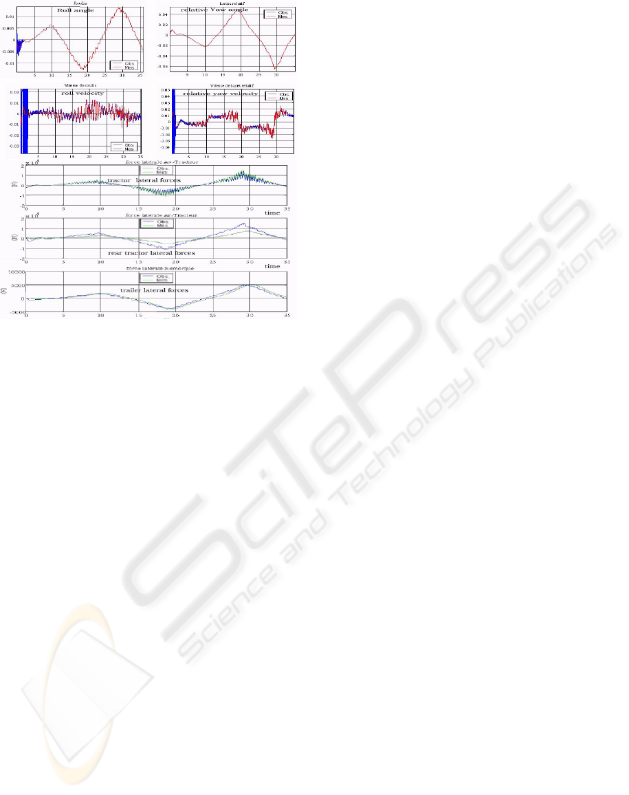
Figure 3: Steering angle and the corresponding motions
(roll, yaw).
4 SIMULATION RESULTS
Some simulations have been done to test and validate
our approach. The forces are generated by use of the
Magic Formula tire model (Pacejka and Besselink,
1997). The input (Steering angle) of model applied
is in figure (3). The Observer Parameters :α
1
=
1.00, α
2
= 1.02, λ
1
= 2.6104, and λ
2
= 2.6103, for
sampling we use δ = 0.00001. The performance of
the observer is shown in figures (3 and ??). The per-
formance of this estimation approach is satisfactory
since the estimation error is minimal for state vari-
ables. So, the unknown parameters converge to their
values.
5 CONCLUSION
This paper presents a new observation and estimation
approach suitable for heavy vehicle. We estimate the
lateral forces using observer based first and second-
order sliding mode algorithm. The finite time conver-
gence of the observer is useful for robustness of the
forces retrieval. Simulations illustrate the ability of
this approach to give estimation of both vehicle dy-
namics states and lateral tire forces. The robustness
of the twisting algorithm versus uncertainties on the
model parameters has also been emphasized.
REFERENCES
Ackermann, J. (1998). Active steering for better safety, han-
dling and comfort. In Advances in Vehicle control and
Safety AVCS’98, Amiens,France.
C.Chen, M. T. (1997). Modelling and control of articu-
lated vehicles. Technical Report UCB-ITS-PRR-97-
42, University of California, Berkeley.
Dahlberg, E. (2001). Commercial Vehicle Stability – Focus-
ing on Rollover. PhD thesis, Royal Institute of Tech-
nology.
Desfontaines, H. (2004). CEESAR: (european center for
safety studies and risk analysis) number = Advanced
Engineering Lyon and Report L1a, Th
`
eme 11; AR-
COS 2004, note = RENAULT TRUCKS, institution =
RVI, Renault V
´
ehicules Industriels. Technical report.
Fillipov, A. (1960). ”Differential Equations with Disconti-
nous Right-Hand Sides”, volume 62.
J. Davila, L. F. (2004). Observation and identification of
mechanical systems via second order sliding modes.
M’Sirdi, N., Manamani, N., and El Ghanami, D. (2000).
Control approach for legged robots with fast gaits:
Controlled limit cycles.
M’sirdi, N., Rabhi, A., Fridman, L., Davila, J., and Delanne,
Y. (2006). Second order sliding-mode observer for
estimation of vehicle parameters. Submitted to IEEE
TCST, page octobre 2005. IEEE Transactions on Con-
trol Systems Technology.
N.K. M’sirdi, A. Rabhi, N. Z. and Delanne, Y. (2004).
VRIM: Vehicle road interaction modelling for estima-
tion of contact forces. In of Vienna Austria, T. U.,
editor, TMVDA 3rd Int. Tyre Colloquium Tyre Models
For Vehicle Dynamics Analysis, Vienna. TMVDA.
P. J. Liu, S. Rakheja, A. A. (1997). Detection of dy-
namic roll instability of heavy vehicles for open-loop
rollover control. In SAE. SAE. paper 973263.
Pacejka, H. and Besselink, I. . (1997). Magic formula tyre
with transient properties. Vehicle System Dynamics
Supplement, 27:234–249.
R. Ervin, C. Winkler, P. F. M. H. V. K. H. Z. S. B. (1998).
Two active systems for enhancing dynamic stability in
heavy truck operations. Technical Report UMTRI-98-
39, UMTRI.
S. Rakheja, A. P. (1990). Evelopment of directional stability
criteria for an early warning safety device. In SAE.
SAE. paper 902265.
Slotine, J., Hedrick, J., and Misawa, E. (1986). Nonlin-
ear state estimation using sliding observers. In Proc.
of 25th IEEE Conference on Decision and Control,
Athen, pages 332–339. Greece.
Utkin, V. I. (1977). Sliding mode and their application in
variable structure systems. Mir, Moscou.
ESTIMATION OF PERFORMANCE OF HEAVY VEHICLES BY SLIDING MODES OBSERVERS
365
