CONTROLLING THE LORENZ SYSTEM WITH DELAY

Yechiel J. Crispin

Department of Aerospace Engineering

Embry-Riddle University, Daytona Beach, FL 32114, USA

Keywords:

Adaptive Control, Chaos, Hyperchaos, Parameter Estimation, Signal Processing, Lagrangian Fluid Dynamics,

Chaotic Advection, Nonlinear Dynamics, Nonlinear Systems and Modeling.

Abstract:

A generalized method for adaptive control, synchronization of chaos and parameter identiﬁcation in systems

governed by ordinary differential equations and delay-differential equations is developed. The method is

based on the Lagrangian approach to ﬂuid dynamics. The synchronization error, deﬁned as a norm of the

difference between the state variables of two similar and coupled systems, is treated as a scalar ﬂuid property

advected by a ﬂuid particle in the vector ﬁeld of the controlled response system. As this error property is

minimized, the two coupled systems synchronize and the time variable parameters of the driving system are

identiﬁed. The method is applicable to the ﬁeld of secure communications when the variable parameters of the

driver system carry encrypted messages. The synchronization method is demonstrated on two Lorenz systems

with variable parameters. We then apply the method to the synchronization of hyperchaos in two modiﬁed

Lorenz systems with a time delay in one the state variables.

1 INTRODUCTION

In this paper we develop a generalized method for

controlling chaos in dynamical systems and for syn-

chronizing two coupled chaotic or hyperchaotic sys-

tems. The systems are described by ordinary dif-

ferential equations with initial conditions or delay-

differential equations with initial functions. The in-

dependent parameters appearing in the equations can

be constant or variable. The synchronization error ,

deﬁned as a norm of the difference between the state

variables of the two chaotic systems, is viewed as

a ﬂuid property advected by a marker particle mov-

ing along a trajectory in the vector ﬁeld of the re-

sponse system. The controlled parameters of the re-

sponse system are varied continuously such as to min-

imize the synchronization error while the two chaotic

systems evolve in time. For the initial value prob-

lem, we derive a system of differential equations gov-

erning the evolution of the controlled parameters re-

quired for synchronization. For the case of the ini-

tial function problem, we derive a system of delay-

differentialequations governing the controlled param-

eters for synchronizing the response system. In both

cases, the ﬂuid dynamical approach mentioned above

is used to develop the equations for the controlled pa-

rameters.

The method is demonstrated by studying sev-

eral examples of chaotic and hyperchaotic systems.

The synchronization method is demonstrated on two

Lorenz systems with variable parameters. We then

apply the method to the synchronization of hyper-

chaos in two modiﬁed Lorenz systems with a time

delay in one the state variables.

The possibility of synchronizing two chaotic phys-

ical systems has attracted considerable attention in re-

cent years (Boccaletti, Farini and Arecchi, 1997). A

major motivation is the potential of applying the syn-

chronization methods to the ﬁeld of secure communi-

cations by chaotic masking or scrambling of messages

(Goedgebuer, Larger and Porte, 1998), (Yang, 2004).

Other important applications are in the ﬁeld of nonsta-

tionary time series analysis and system identiﬁcation

(Parlitz, 1996), (Crispin, 2002). So far, most of the

attention has been directed towards the study of sta-

tionary chaotic systems, that is systems with constant

parameters. To date, the possibility of using systems

with nonstationary parameters for secure communi-

cations has received less attention, although such sys-

tems are good candidates for secure communications,

J. Crispin Y. (2006).

CONTROLLING THE LORENZ SYSTEM WITH DELAY.

In Proceedings of the Third International Conference on Informatics in Control, Automation and Robotics, pages 3-10

DOI: 10.5220/0001219400030010

 SciTePress

especially when the nonstationary parameters rather

than the state variables are used to hide the secret mes-

sages (Crispin, 1998).

Several methods for the control of chaos in dynam-

ical systems have been proposed in recent years (Boc-

caletti et al., 2000). The conjecture of chaos control

by means of perturbations of an accessible parameter

is based on an inherent property of chaotic systems,

namely, their sensitivity to small perturbations in the

parameters (Parlitz, Junge and Kocarev, 1996), (Carr

and Schwartz, 1994), (Ott and Spano, 1995).

Model reference adaptive control methods have

been suggested for chaos suppression and synchro-

nization (Aguirre and Billings, 1994). For example,

a model reference method for the adaptive control

of chaos in dynamical systems with periodic forcing

has been proposed by (Crispin and Ferrari, 1996).

Adaptive control and synchronization of chaos in

discrete time systems has been studied by (Crispin,

1997). Another method for controlling chaos in dy-

namical systems is by introducing parametric forc-

ing and adaptive control, see for example (Crispin,

2000). A more recent method based on an analogy

from ﬂuid dynamics has been described by (Crispin,

2002). Other applications include parameter esti-

mation (Parlitz, Junge and Kocarev, 1996), synchro-

nization of chaotic systems with variable parameters

(Crispin, 1998) and the control of chaos in ﬂuids

(Crispin, 1999).

Many physical, physiological and biological sys-

tems display time delay in their dynamics. Nonlinear

dynamical systems with time delay can have periodic

orbits or very complex dynamics depending upon the

range of values of the time delay and the indepen-

dent parameters of the system. This complex be-

havior has attracted a lot of interest in the study of

time delayed systems from the mathematical point of

view (Kolmanovskii and Myshkis, 1992) as well as

from the physical and physiological points of view,

see for example (Losson, Mackey and Longtin, 1993),

(Mansour and Longtin, 1998). The use of time delay

in feedback control systems has also been proposed,

see for example (Hegger et al., 1998), (Goedgebuer,

Larger and Porte, 1998) and (Just et al., 1998). Con-

trol of chaos in systems with time delay has also been

studied in (Mansour and Longtin, 1998).

2 THE FLUID DYNAMICAL

APPROACH

Consider two similar dynamical systems described by

ordinary differential equations. We deﬁne two dy-

namical systems as similar if the right hand sides of

the equations are represented by the same function

f(x(t), p(t)), except that the independent parameters

p(t) or q(t) can be represented either by different

or the same functions of time. We ﬁrst present the

method for the initial value problem and then we con-

sider the case when one of the state variables has a

time delay.

dx/dt = f (x(t), p(t)) (2.1)

dy/dt = f(y(t), q(t))

Here t is time, x ∈R

are the state variables of

the driver and y ∈R

are the state variables of

the response system. The parameters p(t) ∈R

and

q(t) ∈R

are independent time variable parameters

of the respective systems and f :R

x R

7→R

a nonlinear vector function of the state variables. It

is assumed that the initial values of the state variables

x(0) = x

and y(0) =y

for t = 0 are not neces-

sarily the same. Similarly the initial values of the pa-

rameters p(0) = p

and q(0) = q

of the driver

and response systems are different. Since chaotic sys-

tems are sensitive to initial conditions, the driver and

response systems will not synchronize, unless the re-

sponse system is controlled and forced to synchronize

with the driver system using some kind of coupling,

such as a transmitted scalar signal. For instance, a sin-

gle scalar signal s(t), which is a function of the state

x(t), can be transmitted by the driver and used to en-

slave the response system (Tamasevicius and Cenys,

1997), (Peng, Ding and Yang, 1996).

s(t) = h(x(t)) (2.3)

As stated above, the purpose of this paper is to

propose a generalized method of control, stabiliza-

tion, synchronization and parameter identiﬁcation of

chaotic systems in the more general case where the

parameters p(t) of the driver system vary as a func-

tion of time. In the context of secure communica-

tions, this means that it would be possible to encode a

message in one of the parameters of the driver system

rather then in a state variable, as has been proposed

so far. Once a variable parameter is identiﬁed by

the response system using the proposed generalized

method, the encoded message can be recovered. The

method allows more ﬂexibility in masking informa-

tion in chaos. The message can be encoded in a state

variable or in a time variable parameter. The useful in-

formation can also be split into two messages, where

one message is modulated by a state variable and a

second message modulated by a parameter. Synchro-

nization of the state variables of an eavesdropping re-

sponse system with the state variables of the driver

will be difﬁcult because of the sensitivity to small

variations in the parameters of the system, in addition

to the sensitivity to initial conditions and the diver-

gence of nearby trajectories in chaotic systems. Also,

ICINCO 2006 - SIGNAL PROCESSING, SYSTEMS MODELING AND CONTROL

synchronization can be achieved even when the pa-

rameters p(t) and q(t) are initially substantially dif-

ferent. This is accomplished by controlling the re-

sponse system y such that the parameters p(t) of the

driver system x are eventually identiﬁed, that is,

lim

t→∞

|p(t) − q(t)| = 0 (2.4)

In order to achieve synchronization, the dynamics

of the response system parameters q(t) need to be

determined. In other words, the differential equations

governing the evolution of the response parameters

q(t) need to be derived for dynamical systems of the

form of Eqs.(2.1-2.2).

The proposed ﬂuid dynamical approach is based on

the Lagrangian description of ﬂuid motion. It fol-

lows the motion of a ﬂuid particle as it moves in

the velocity vector ﬁeld w(x, p) created by a ﬂuid

ﬂow (Lamb, 1995), (Milne-Thomson, 1968). Ac-

cording to this approach, the equations of motion of

two marker particles advected in the ﬂuid ﬂows de-

scribed by the vector ﬁelds w(x, p) = f (x, p) and

w(y, q) = f(y, q), are given by Eq.(2.1-2.2), where

the right hand sides are to be interpreted as the lo-

cal velocity vectors w(x, p) and w(y, q) at any given

point x ∈R

and y ∈R

of the two ﬂow ﬁelds, re-

spectively, i.e,

dx/dt = w(x, p) = f (x, p) (2.5)

dy/dt = w(y, q) = f (y, q)

In ﬂuid dynamics, the vector ﬁelds

w(x, p), w(y, q) ∈R

and the state variables

x, y ∈R

have a dimension n ≤ 3. Here the analogy

is extended to vector ﬁelds of higher dimensions.

Consider the time variation of a scalar property

J(x, y) of the ﬂow along a trajectory of the response

system as it evolves in the state space y ∈R

. The

rate of change of this scalar property is due to two

contributions: a local contribution due to its time

variation, plus a contribution which is due to the rate

of change of the property as it is advected along the

trajectory in the state space. The total rate of change

is then given by the substantial derivative DJ/Dt

of the scalar property J, which is the derivative

following the ﬂow:

DJ/Dt = ∂J/∂t + f (y(t), q)∇J (2.6)

∇ = (∂/∂y

, ∂/∂y

, ..., ∂/∂y

)

Here the product f (y, q)∇J is a scalar or dot

product. Consider a scalar property J based on the

Euclidean distance between the state vectors x and

y :

J =

|y −x|

i=1

−x

)

i=1

(2.7)

where e

= y

− x

are components of the error

vector function e = y − x . Using Eq.(2.7), the local

component of the derivative of J with respect to time

is given by:

∂J/∂t =

i=1

/dt (2.8)

whereas the components of the gradient ∇J are

given by

∂J/∂y

= y

− x

= e

(2.9)

Using Eqs.(2.5), (2.6), (2.8) and (2.9), the substan-

tial derivative of J is written as:

DJ/Dt =

i=1

[de

/dt + f

(y(t), q)] (2.10)

and since e = y − x and

de/dt = dy/dt − dx/dt = f (y, q) − f(x, p)

Eq.(2.10) reduces to:

DJ/Dt =

i=1

[2f

(y(t), q) −f

(x(t), p)] (2.11)

Eq.(2.11) deﬁnes the rate of change of the positive

scalar property J in terms of the state variables x and

y of the driver and response systems, the independent

driver parameters p and the controllable parameters

q of the response system. The question now is how

should the control vector q be varied such as to con-

tinuously minimize J? As the driver and response

systems evolve, the substantial derivative should be

continuously decreased in order to achieve control

and synchronization, as can be seen from Eq.(2.11),

where perfect synchronization is reached when e =

y − x = 0, and from Eq.(2.7), J reaches the mini-

mum J = 0. A possible control law is to vary the

control vector q such as to decrease the substantial

derivativeDJ/Dt, that is, to continuously change the

control q in a direction opposite to the gradient of

DJ/Dt with respect to the control q:

dq/dt = −G

′

∇

(DJ/Dt) =

= −G

′

∇

{

i=1

[2f

(y(t), q) − f

(x(t), p)]}

(2.12)

CONTROLLING THE LORENZ SYSTEM WITH DELAY

where

∇

= (∂/∂q

, ∂/∂q

, ..., ∂/∂q

)

and G

′

is a kxk matrix of control gains. Since

(x, p) does not depend on the control q ,it follows

that

∇

(x(t), p) = 0

and Eq.(2.12) becomes:

dq/dt = −G ∇

[

i=1

(y(t), q)] (2.13)

where G = 2G

′

3 SYNCHRONIZING THE

LORENZ SYSTEM

We now apply the method to a dynamical system

without delay, the chaotic Lorenz system. Consider

the case of synchronization between two Lorenz sys-

tems with variable parameters, where the driver sys-

tem is given by:

/dt = σ(x

− x

)

/dt = p

(t)x

− p

(t)x

− p

(t)x

(3.1)

/dt = x

− bx

and the transmitted coupling signal for synchro-

nization is chosen as the single variable:

s(t) = h(x(t)) = x

(t) (3.2)

The response system is deﬁned by the following

Lorenz system with variable parameters. It is driven

by the transmitted signal s(t) = x

(t).

/dt = σ(s(t) − y

)

/dt = q

(t)y

− q

(t)y

− q

(t)y

(3.3)

/dt = y

s(t) − by

The next step is to derive a system of differen-

tial equations governing the evolution of the con-

trolled parameters q

(t), q

(t) and q

(t). As the

response system evolves and synchronizes with the

driver system, the parameters q

(t), q

(t) and q

(t)

will follow the original parameters p

(t), p

(t) and

(t) of the driver system. According to Eq.(2.13) of

the previous section, the ﬁrst step is to develop the

term

i=1

(y, q) for the response system (3.3).

Using the right hand sides of (3.3), we have:

i=1

(y, q) = (y

− x

)[σ(s(t) − y

)]+

+(y

− x

)[q

(t)y

− q

(t)y

− q

(t)y

+(y

− x

)(y

s(t) − by

) (3.4)

The gradient with respect to the parameters q is

given by:

∇

[

i=1

(y, q)] =

= [(y

− x

, −(y

− x

, −(y

− x

]

(3.5)

The differential equations governing the evolution

of the controlled parametersq are given by:

/dt = −G

− s(t))y

+ G

− s(t))y

/dt = −G

− s(t))y

+ G

− s(t))y

(3.6)

/dt = −G

− s(t))y

+ G

− s(t))y

For example, consider the case where only one pa-

rameter, say p

(t) is to be identiﬁed, whereas the

other two parametersp

(t) and p

(t) are known con-

stants. If the synchronized systems are used for se-

cure communication, the parameter p

(t) can be used

to carry a hidden message, which can be identiﬁed by

the response system. In this case, Equations (3.4-3.6)

reduce to:

i=1

(y, q) = (y

− x

)[σ(s(t) − y

)]+

+(y

− x

)[q

(t)y

− p

(t)y

− p

(t)y

ICINCO 2006 - SIGNAL PROCESSING, SYSTEMS MODELING AND CONTROL

+(y

− x

)(y

− by

) (3.7)

∇

[

i=1

(y, q)] = [(y

− x

, 0 , 0]

(3.8)

/dt = −G

− s(t))y

(3.9)

/dt = 0

We now show results of a computer simulation with

the following values of the parameters:

σ = 10 b = 8/3 (3.10a)

(t) = r

+ δr sin ωt (3.10b)

δr = 2 ω = 2π/10 r

= 28 (3.10c)

= p

= 1 q

= p

= 1 (3.10d)

together with the initial condition:

(0) = r

= 28 (3.10e)

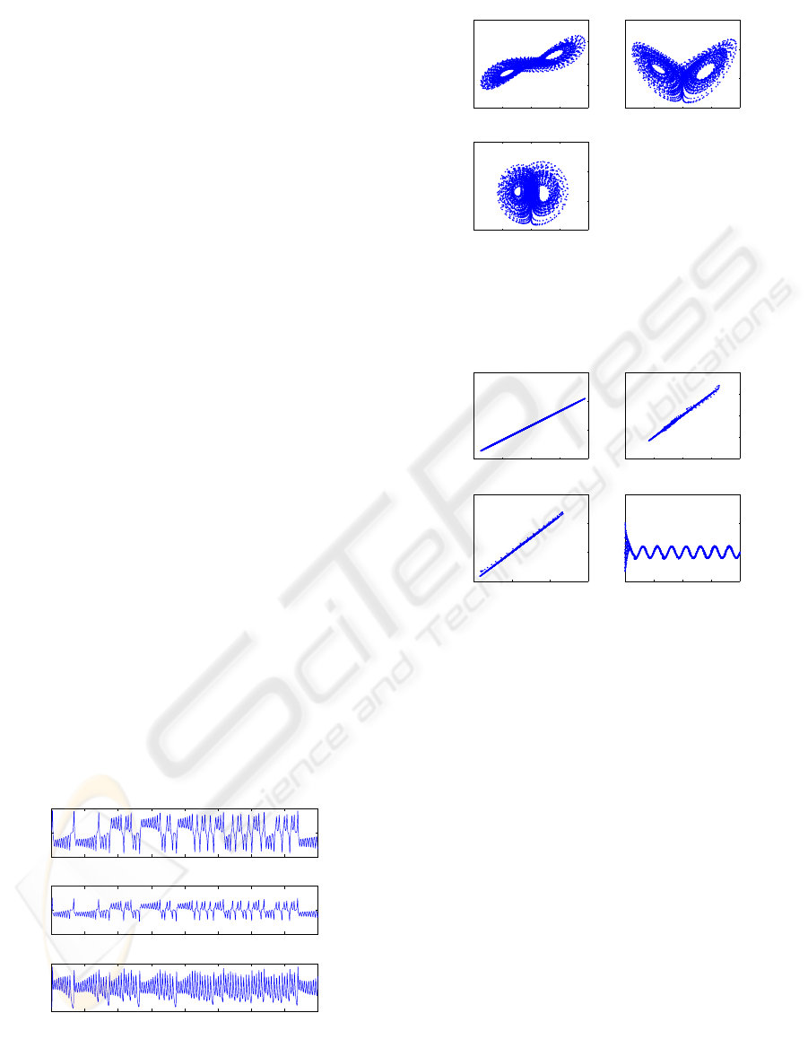
The results of this example are given in Figures

1-3. Fig.1 shows the chaotic state variables of the

driver system. The chaotic attractor is shown in Fig.2.

Similar results are obtained for the response system

as it synchronizes with the driver system. Fig.3 dis-

plays the synchronized state variables y

= x

andy

= x

, all three eventually converging to

straight lines as shown in the ﬁgure. The identi-

ﬁed signal q

(t) − r converges to the driver signal

(t) − r = δr sin ωt and is also shown in the ﬁgure.

0 10 20 30 40 50 60 70 80

−20

0 10 20 30 40 50 60 70 80

−50

0 10 20 30 40 50 60 70 80

Figure 1: The chaotic state variables of the driver Lorenz

system with variable parameter.

−20 −10 0 10 20

−40

−20

−20 −10 0 10 20

−40 −20 0 20 40

Figure 2: The chaotic attractor of the driver Lorenz system

with variable parameter. The response system has a similar

attractor.

−20 −10 0 10 20

−20

−40 −20 0 20 40

−40

−20

0 20 40 60

0 20 40 60 80

−10

q1 − r

Figure 3: Synchronization between the driver and response

Lorenz systems with variable parameters and the parameter

(t) of the response system as it identiﬁes the driver signal

(t).

4 SYNCHRONIZING LORENZ

SYSTEM WITH DELAY

In this section we apply the method to a hyperchaotic

dynamical system, the Lorenz system with a time de-

lay in one of the state variables. Consider the case

of synchronization between two Lorenz systems with

time delay. We treat the case where the state variable

(t − T ) is delayed by a time delay T . Here the

driver system is given by:

/dt = σ(x

(t) − x

(t − T ))

/dt = p

(t)x

(t − T ) − p

(t)x

(t)−

−p

(t)x

(t − T )x

(t)

/dt = x

(t − T )x

(t) − bx

(t) (4.1)

CONTROLLING THE LORENZ SYSTEM WITH DELAY

Suppose the transmitted signal for synchronization

is chosen as the single variable:

s(t) = h(x(t)) = x

(t) (4.2)

The response system is deﬁned by the following

nonstationary and delayed Lorenz system, where the

transmitted scalar signal s(t) = x

(t) is used to drive

the system.

/dt = σ(s(t) − y

(t − T ))

/dt = q

(t)y

(t − T ) − q

(t)y

(t)−

−q

(t)y

(t − T )y

(t)

/dt = y

(t − T )s(t) − by

(t) (4.3)

The next step is to derive a system of differential

equations governing the evolution of the controlled

parameters q

(t), q

(t) and q

(t). As the response

system evolves and synchronizes with the driver sys-

tem, the parameters q

(t), q

(t) and q

(t) will follow

the original parameters p

(t), p

(t) and p

(t) of the

driver system. According to Eq.(2.13) of section 2,

the ﬁrst step is to develop the term

i=1

(y, q)

for the response system (4.3).

i=1

(y, q) = (y

(t − T ) − x

)[σ(s(t) − y

(t − T ))]+

+(y

− x

)[q

(t)y

(t− T )− q

(t)y

− q

(t)y

(t− T )y

+(y

− x

)[y

(t − T )s(t) − by

] (4.4)

The gradient with respect to the parameters q is

given by:

∇

[

i=1

(y, q)] =

= [(y

− x

(t − T ) , −(y

− x

, −(y

− x

(t − T )y

]

(4.5)

The differential equations governing the evolution

of the controlled parametersq are given by:

/dt = −G

− s(t))y

(t− T )+G

− s(t))y

(t − T )y

/dt = −G

− s(t))y

(t− T )+G

− s(t))y

(t − T )y

/dt = −G

− s(t))y

(t− T )+G

− s(t))y

(t − T )y

(4.6)

For example, consider the case where only one pa-

rameter, say p

(t) is to be identiﬁed, whereas the

other two parametersp

(t) and p

(t) are known con-

stants. If the synchronized systems are used for secure

communication, the parameter p

(t) can carry a hid-

den message, which can be identiﬁed by the response

system. In this case, Equations (4.4-4.6) reduce to:

i=1

(y, q) = (y

− x

)[σ(s(t) − y

)]+

+(y

−x

)[q

(t)y

−p

]+(y

−x

)(y

−by

)

(4.7)

∇

[

i=1

(y, q)] = [(y

− x

(t − T ), 0 , 0]

(4.8)

/dt = −G

− s(t))y

(t − T ) (4.9)

/dt = 0

Here we show results of a computer simulation

with the following values of the parameters:

σ = 10 b = 8/3 T = 0.1 G11 = 10 (4.10a)

(t) = r

+ δr sin ωt (4.10b)

δr = 2 ω = 2π/10 r

= 28 (4.10c)

= p

= 1 q

= p

= 1 (4.10d)

together with the initial condition:

(0) = r

= 28 (4.10e)

The results of this example are given in Figures 4-

6. Fig.4 shows the hyperchaotic state variables of the

driver system. A comparison with Fig.1 above, it can

be seen that the state variables in Fig.4 display a more

complex type of chaos, because of the time delay.

ICINCO 2006 - SIGNAL PROCESSING, SYSTEMS MODELING AND CONTROL

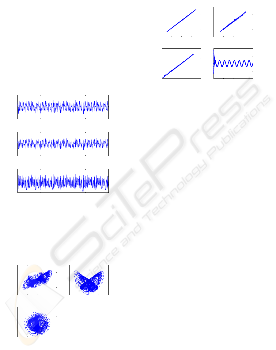
Comparing with the attractor of Fig. 2 above, it is ap-

parent that the hyperchaotic attractor shown in Fig.5

displays a more complex behavior. Similar results are

obtained for the response system as it synchronizes

with the driver system. Fig.6 displays the synchro-

nized state variables y

= x

andy

= x

all three eventually converging to straight lines as

shown in the ﬁgure. The identiﬁed signal q

(t) − r

converges to the driver signal q

(t) − r = δr sin ωt

and is also shown in the ﬁgure.

0 20 40 60 80

−50

0 20 40 60 80

−50

0 20 40 60 80

Figure 4: The hyperchaotic state variables of the driver

Lorenz system with delay and variable parameter.

−40 −20 0 20 40

−40

−20

−40 −20 0 20 40

Figure 5: The hyperchaotic attractor of the driver Lorenz

system with delay and variable parameter. The response

system has a similar attractor.

−40 −20 0 20 40

−40

−20

−40 −20 0 20 40

−40

−20

0 20 40 60

0 20 40 60 80

−10

−5

q1 − r

Figure 6: Synchronization between the hyperchaotic driver

and response Lorenz systems with delay and variable pa-

rameters and the parameter q

(t) of the response system as

it identiﬁes the driver signal p

(t).

5 CONCLUSIONS

A generalized method for adaptive control, synchro-

nization of chaos and parameter identiﬁcation in sys-

tems governed by ordinary differential equations and

delay-differential equations has been presented. The

method is based on the Lagrangian approach to ﬂuid

dynamics. The synchronization error is treated as a

scalar ﬂuid property advected in the vector ﬁeld of the

controlled response system. Upon minimizing this er-

ror, the two coupled systems synchronize and the time

variable parameters of the driving system are identi-

ﬁed. The method was used to synchronize two Lorenz

systems with variable parameters. The method was

also applied to the synchronization of hyperchaos in

two modiﬁed Lorenz systems with a time delay in one

the state variables. Some implications of using the

method in the ﬁeld of secure communications where

the transmitted information is masked by chaos or hy-

perchaos have been discussed.

REFERENCES

Aguirre, L. and Billings, S. (1994). Model Reference Con-

trol of Regular and Chaotic Dynamics in the Dufﬁng-

Ueda Oscillator. In IEEE Transactions on Circuits and

Systems I, 41, 7, 477-480. IEEE.

Boccaletti, S., Farini, A. and Arecchi, F.T. (1997). Adaptive

Synchronization of Chaos for Secure Communication.

In Physical Review E, 55, 5, 4979-4981.

Boccaletti, S., Grebogi, C., Lai, Y.C., Mancini, H. and

Maza, D. (2000). The Control of Chaos: Theory and

Applications. In Physics Reports 329, 103-197, Else-

vier.

Carr, T. and Schwartz, I. (1994). Controlling Unstable

Steady States Using System Parameter Variation and

CONTROLLING THE LORENZ SYSTEM WITH DELAY

Control Duration. In Physical Review E, 50, 5, 3410-

3415.

Crispin, Y. (2002). A Fluid Dynamical Approach to the

Control, Synchronization and Parameter Identiﬁcation

of Chaotic Systems. In American Control Conference,

ACC 2002, Anchorage, AK, 2245-2250.

Crispin, Y. (2000) Controlling Chaos by Adaptive Para-

metric Forcing. In Intelligent Engineering Systems

Through Artiﬁcial Neural Networks, Vol. 10, Edited

by Dagli et al., ASME Press, New York.

Crispin, Y. (1999) Control and Anticontrol of Chaos in Flu-

ids. In Intelligent Engineering Systems Through Arti-

ﬁcial Neural Networks, Vol. 9, Edited by Dagli et al.,

ASME Press, New York.

Crispin, Y. (1998). Adaptive Control and Synchronization

of Chaotic Systems with Time Varying Parameters.

In Intelligent Engineering Systems Through Artiﬁcial

Neural Networks, Vol. 8, Edited by Dagli et al., ASME

Press, New York.

Crispin, Y. (1997) Adaptive Control and Synchronization of

Chaos in Discrete Time Systems. In Intelligent Engi-

neering Systems Through Artiﬁcial Neural Networks,

Vol. 7, Edited by Dagli et al., ASME Press, New York.

Crispin, Y. and Ferrari, S. (1996). Model Reference Adap-

tive Control of Chaos in Periodically Forced Dynami-

cal Systems. In 6th AIAA/USAF/NASA Symposium on

Multidisciplinary Analysis and Optimization, Belle-

vue, WA, 882-890, AIAA Paper 96-4077.

Goedgebuer, J.P., Larger, L. and Porte, H. (1998). Opti-

cal Cryptosystem Based on Synchronization of Hy-

perchaos Generated by a Delayed Feedback Tunable

Laser Diode. In Physical Review Letters, 80, 10,

pp.2249-2252.

Hegger, R., Bunner M.J., Kantz, H. and Giaquinta, A.

(1998) Identifying and Modeling Delay Feedback

Systems. In Physical Review Letters, 81, 3, 558-561.

Just, W., Reckwerth, D., Mockel, J., Reibold, E. and H.

Benner, H. (1998) Delayed Feedback Control of Peri-

odic Orbits in Autonomous Systems. In Physical Re-

view Letters, 81, 3, 562-565.

Kolmanovskii, V. and A. Myshkis, A. (1992) Applied The-

ory of Functional Differential Equations. In Math-

ematics and its Applications, Vol. 85, Kluwer, Dor-

drecht.

Lamb, H. (1995). Hydrodynamics. Cambridge University

Press, NY, sixth edition.

Losson, J, Mackey, M.C. and Longtin, A. (1993). Solu-

tion Multistability in First-order Nonlinear Differen-

tial Delay Equations. In Chaos, 3, 2, 167-176.

Mansour, B. and Longtin, A. (1998) Chaos Control in Mul-

tistable Delay Differential Equations and Their Singu-

lar Limit Maps. In Physical Review E, 58, 1, 410-422.

Mansour, B. and A. Longtin, A. (1998) Power Spectra and

Dynamical Invariants for Delay Differential and Dif-

ference Equations. In Physica D 113, 1, 1-25.

Milne-Thomson, L. (1968). Theoretical Hydrodynamics.

MacMillan, NY, ﬁfth edition.

Ott, E. and Spano, M. (1995). Controlling Chaos. In Physics

Today, 48, 34.

Parlitz, U. (1996). Estimating Model Parameters From

Time Series by Auto-Synchronization. In Physical

Review Letters, 76, 8, pp.1232-1235.

Parlitz, U., Junge, L. and Kocarev, L. (1996). Synchroniza-

tion Based Parameter Estimation From Time Series.

In Physical Review E, 54, 6, pp.6253-6259.

Peng, J.H., Ding, E.J., Ding, M. and Yang, W. (1996). Syn-

chronizing Hyperchaos with a Scalar Transmitted Sig-

nal. In Physical Review Letters, 76, 6, 904-907.

Tamasevicius, A. and Cenys, A. (1997). Synchronizing Hy-

perchaos with a Single Variable. In Physical Review

E, 55,1, 297-299.

Yang, T. (2004). A Survey of Chaotic Secure Communica-

tion Systems. In International Journal of Computa-

tional Cognition, 2, 2, 81-130.

ICINCO 2006 - SIGNAL PROCESSING, SYSTEMS MODELING AND CONTROL