NEURO-ADAPTIVE DYNAMIC CONTROL FOR TRAJECTORY

TRACKING OF MOBILE ROBOTS

Marvin K. Bugeja† and Simon G. Fabri‡

Department of Electrical Power and Control Engineering, University of Malta

Msida MSD06, Malta

Keywords:

Nonholonomic mobile robots, trajectory tracking, adaptive control, neural networks, stochastic estimation.

Abstract:

This paper presents a novel functional-adaptive dynamic controller for trajectory tracking of nonholonomic

wheeled mobile robots. The controller is developed in discrete-time and employs a Gaussian radial basis

function neural network for the estimation of the robot’s nonlinear dynamic functions, which are assumed

to be completely unknown. Optimal on-line weight tuning is achieved by employing the Kalman ﬁlter algo-

rithm, based on a speciﬁcally formulated stochastic inverse dynamic identiﬁcation model of the mobile base.

A discrete-time dynamic control law employing the estimated functions is proposed and cascaded with a tra-

jectory tracking kinematic controller. The performance of the complete system is analysed and compared by

realistic simulations.

1 INTRODUCTION

Motion control of nonholonomic mobile robots has

been receiving considerable attention for the last ﬁf-

teen years (Kolmanovsky and McClamroch, 1995).

This activity is not only justiﬁed by the vast array

of existing and potential practical applications (Lami-

raux et al., 2005; Ding and Cooper, 2005), but also by

some particularly interesting theoretical challenges.

In particular, most mobile conﬁgurations manifest re-

stricted mobility; giving rise to nonholonomic con-

straints in the kinematics. Moreover the majority of

mobile vehicles are underactuated, since they have

more degrees of freedom than control inputs. Con-

sequently the linearised kinematic model lacks con-

trollability, full-state feedback linearisation is out of

reach (Canudas de Wit et al., 1993), and pure, smooth,

time-invariant feedback stabilisation of the Cartesian

kinematic model is unattainable (Brockett, 1983).

Originally researchers focused only on kinematic

control of nonholonomic vehicles (Crowley, 1989;

Kanayama et al., 1990; Canudas de Wit et al., 1993;

Kolmanovsky and McClamroch, 1995), assuming

that the control signals instantaneously establish the

desired robot velocities. This is commonly known

as perfect velocity tracking(Fierro and Lewis, 1995).

This approach may be reasonably valid for light ro-

bots following low acceleration trajectories. How-

ever it stands to reason that controllers based on a

full dynamic model (Sarkar et al., 1994; Fierro and

Lewis, 1995; Corradini and Orlando, 2001) capture

better the behaviour of real robots because they ac-

count for dynamic effects such as mass, friction and

inertia, which are otherwise neglected by a mere kine-

matic controller. On the other hand, the exact val-

ues of the parameters in the dynamic model are often

uncertain or even unknown, and may even vary over

time. A typical case is that of a mobile robot carrying

unspeciﬁed loads, and/or moving on several surfaces

with different frictional conditions.

These factors call for the development of adap-

tive dynamic controllers to better handle unmod-

elled robot dynamics, as well as noise and exter-

nal disturbances. Addressing of these advanced con-

trol issues of robustness and adaptation for the dy-

namic/kinematic control of nonholonomic mobile ro-

bots is a recent development. Some researchers opt to

use pre-trained function estimators, speciﬁcally arti-

ﬁcial neural networks (ANNs), to render nonadaptive

conventional controllers more robust in the face of un-

certainty (Corradini et al., 2003; Oubbati et al., 2005).

These techniques require prior off-line training and

remain blind to variations and situations which take

place after the training phase. In contrast to the claim

in (Oubbati et al., 2005) such techniques cannot be

considered as adaptive because this requires real-time

404

Bugeja M. and Fabri S. (2006).

NEURO-ADAPTIVE DYNAMIC CONTROL FOR TRAJECTORY TRACKING OF MOBILE ROBOTS.

In Proceedings of the Third International Conference on Informatics in Control, Automation and Robotics, pages 404-411

DOI: 10.5220/0001218904040411

 SciTePress

and continuous online training. To account for para-

metric variations in the kinematic/dynamic model,

adaptive control (Fukao et al., 2000) and robust slid-

ing mode control (Corradini and Orlando, 2001) has

also been proposed. Yet another approach is that of

online functional-adaptive control, where the uncer-

tainty is not restricted to parametric terms, but cov-

ers also the dynamic functions themselves. We con-

sider this to be more general and superior in handling

higher degrees of uncertainty and unmodelled dynam-

ics (Fierro and Lewis, 1998; de Sousa et al., 2002;

Bugeja and Fabri, 2005).

In all these works, only Corradini et al. [2003] and

Bugeja and Fabri [2005] develop the corresponding

control algorithms in discrete-time. This is a relevant

contribution because in practice robot controllers are

ultimately implemented digitally on computer hard-

ware. The control algorithm proposed by Corradini et

al. [2003] is however not adaptive since it requires

off-line training. It also considers solely the kine-

matic aspect of nonholonomic mobile robots, as does

the adaptive method proposed by Bugeja and Fabri

[2005]. The control scheme being proposed in this

paper conforms with the discrete-time philosophy of

the previous two papers, but addresses their limita-

tions by proposing online functional adaptive control

of the full dynamic model of the nonholonomic mo-

bile robot.

This paper proposes a Gaussian radial basis func-

tion (RBF) ANN to estimate the robot’s nonlinear

dynamic functions, which are assumed to be com-

pletely unknown. The ANN parameters are estimated

stochastically in real-time with no preliminary off-

line training by employing the Kalman ﬁlter algo-

rithm (Kalman, 1960). The estimated functions are

used on a certainty equivalence (van de Water and

Willems, 1981) basis in a discrete-time dynamic con-

trol law cascaded with a trajectory tracking kinematic

controller. The stochastic nature of the ANN weight

estimator is attractive for two main reasons: it pro-

vides a direct way to account for practically inevitable

process and measurement noise; and it provides a di-

rect measure of the estimation uncertainty through the

Kalman covariance matrix. We plan to use the lat-

ter in the development of stochastic controllers in the

nearby future to avoid certainty equivalence assump-

tions.

Section 2 of this paper will develop the stochas-

tic discrete-time inverse dynamic model of the robot.

This is then utilised for identiﬁcation in the online

stochastic estimator based on a Gaussian RBF ANN

in Section 3. A discrete-time adaptive control law is

proposed and incorporated with the recursive weight

tuning algorithm in Section 4. The performance of

the complete system is analysed and compared by re-

alistic simulation results in Section 5, and conclusions

are provided in Section 6.

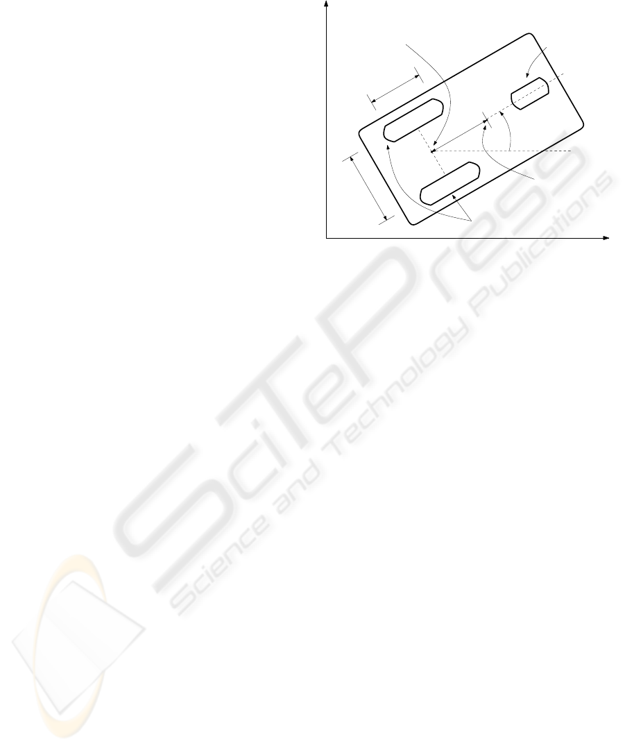
2 PRELIMINARIES

Driving wheels

Passive

wheel

Centre of

mass

Geometric

centre

Figure 1: Differentially driven wheeled mobile robot.

This paper considers the differentially driven wheeled

mobile platform depicted in Figure 1. We ignore the

passive wheel and adopt the following notation.

: midpoint between the two wheels

: centre of mass of the platform without wheels

d: distance from P

to P

b: distance from each wheel to P

r: radius of each wheel

: mass of the platform without wheels

: mass of each wheel

: moment of inertia of the platform about P

: moment of inertia of wheel about its axle

: moment of inertia of wheel about its diameter

The robot dynamic state can be expressed as a

ﬁve dimensional vector q , [x y φ θ

]

, where

(x, y) is the coordinate of P

, φ is the robot orien-

tation angle with reference to the xy frame, θ

and

are the angular displacements of the right and left

driving wheels respectively. The pose of the robot

refers to the three-dimensional vector p , [x y φ].

2.1 Kinematics

Assuming that the driving wheels roll without slip-

ping, the mobile platform is subject to three kinematic

constraints, two of which are nonholonomic (Sarkar

et al., 1994). The three kinematic constraints can be

written in the form

A(q) ˙q = 0, (1)

where

A =

− sin φ cos φ 0 0 0

cos φ sin φ b −r 0

cos φ sin φ −b 0 −r

. (2)

NEURO-ADAPTIVE DYNAMIC CONTROL FOR TRAJECTORY TRACKING OF MOBILE ROBOTS

405

Furthermore, it is straightforward to verify that

A(q)S(q) = 0 where

S =







cos φ

sin φ

−

1 0

0 1







. (3)

The kinematic state-space model of the wheeled mo-

bile robot (WMR) in Figure 1 can now be expressed

˙q = S(q)ν, (4)

where ν represents a column vector composed of the

angular velocities of the two driving wheels, speciﬁ-

cally ν = [ν

]

2.2 Dynamics

The WMR under consideration is a mechanical sys-

tem with the kinematic constraints given in (1). Its

dynamic equations of motion can be written in matrix

form as (Sarkar et al., 1994):

M(q)¨q+V ( ˙q, q) ˙q+F ( ˙q) = E(q)τ −A

(q)λ, (5)

where M(q) is the inertia matrix, V ( ˙q, q) is the cen-

tripetal and Coriolis matrix, F ( ˙q) is a vector of fric-

tional forces, E(q) is the input transformation matrix,

τ is the input torque vector and λ is the vector of con-

straint forces.

Differentiating (4) with respect to time, substi-

tuting the expression for ¨q in (5), premultiplying

the resulting expression by S

(q), and noting that

(q)A

(q) = 0 we get

M ˙ν + V ( ˙q)ν + F ( ˙q) = Eτ . (6)

It can be shown that:

M =

(mb

+ I) + I

(mb

− I)

(mb

− I)

(mb

+ I) + I

V ( ˙q) =

(7)

F ( ˙q) = S

(q)F ( ˙q)

E =



1 0

0 1



where I = (I

+ m

) + 2(I

+ m

) and

m = m

+ 2m

. From (6) and (7) it is straight-

forward to note that the nonlinearities in the WMR

dynamics can be totally attributed to

V ( ˙q) and F ( ˙q),

since M is a constant matrix. Moreover, it is interest-

ing to note that

M is invertible for all possible values

of the WMR parameters and that

V ( ˙q) is effectively

a function of ν only, since

φ =

(ν

− ν

) as can

be seen in (3) and (4).

We will now discretise the continuous-time dynam-

ics in (6) to account for the fact that the controller

is implemented on a digital computer system. Us-

ing a ﬁrst order explicit forward Euler approximation

with sampling interval T seconds and assuming that

the control input vector τ remains constant over each

sampling interval, the following discrete-time inverse

dynamic model is obtained:

k−1

= f

k−1

+ G (ν

− ν

k−1

) , (8)

where the subscript integer k denotes that the corre-

sponding variable is evaluated at sample time instant

kT seconds. We assume that the sampling interval

is chosen low enough for the Euler approximation to

hold. Vector f

k−1

and matrix G are given as:

k−1

+ F

k−1

G =

M . (9)

To account for noise, uncertainty and disturbances

we introduce additively a vector of discrete white

noise ǫ

. The deterministic model in (8) is hence con-

verted to the following nonlinear, stochastic, discrete-

time inverse dynamic model of the WMR:

k−1

= f

k−1

+ G (ν

− ν

k−1

) + ǫ

, (10)

where ǫ

is assumed to be an independent, zero-mean,

white, Gaussian-distributed process, with covariance

matrix R. Identiﬁcation of this model is described in

the next section.

3 GAUSSIAN RBF ESTIMATOR

Theoretically speaking, at any time instant kT the

vector of discrete functions f

and the constant ma-

trix G, composing the WMR inverse dynamic model

in (10), are both known and given in (9). This is true

if one assumes that: there are no unmodelled dynam-

ics, the robot parameters such as masses, inertias and

frictions are perfectly known and do not change over

time, and that perfect sensor measurements are avail-

able. To conform with these stringent conditions in

a real life scenario is practically impossible. To ad-

dress these issues we opt to use functional-adaptive

control via a RBF ANN for the recursive estimation

of the vector of discrete nonlinear functions f

, as if

it was completely unknown. On the other hand, it is

known that G is a constant and symmetrical matrix

with unknown elements. Consequently its estimation

does not require the use of an ANN, and so we in-

tegrate the estimation of the elements of G within

the same Kalman ﬁlter algorithm used for the ANN

weight training, as detailed later in Subsection 3.1.

ICINCO 2006 - ROBOTICS AND AUTOMATION

406

The selection of a Gaussian RBF network (Pog-

gio and Girosi, 1990) for the estimation of f

, was

motivated by the fact that the RBF network weights

appear linearly in the ﬁnal state-space output equa-

tion (Fabri and Kadirkamanathan, 1998). This de-

tail enables the use of a standard Kalman ﬁlter for

weight estimation, leading to the least-squares-sense

optimal tuning of the network weights. In our pre-

vious work (Bugeja and Fabri, 2005), which dealt

with adaptive kinematic control of WMR, multilayer

perceptron (MLP) ANN were used for the estimation

process. Unlike the Gaussian basis functions in RBFs,

the sigmoidal activation functions used in MLPs are

not localised, implying that typically MLP networks

require less neurons than RBF networks for the same

degree of accuracy. However MLP networks do not

posses the possible advantage of linearity, as in the

case of RBF networks. As a result the former Kalman

ﬁlter has to be replaced by a sub-optimal, nonlinear

stochastic estimator, like the extended Kalman ﬁlter

(EKF) (Maybeck, 1979), which complicates the algo-

rithm and introduces signiﬁcant approximations.

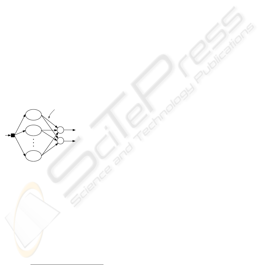
3.1 Formulation







k−1

) ˆw

k−1

) ˆw







k−1







ˆw







Figure 2: RBF neural network.

Consider the following deﬁnitions, in the light of the

employed RBF ANN depicted in Figure 2.

• x

k−1

represents the neural network input vector

deﬁned as:

k−1

, ν

k−1

. (11)

This state vector is assumed to be contained within

the compact set χ

⊂ R

• φ

) is the Gaussian RBF vector, whose ith el-

ement is given by

= exp

(

− m

)

−1

− m

)

−2

)

(12)

where m

is the coordinate vector of the center of

the ith basis function and R

is the corresponding

covariance matrix. The basis functions are placed

on a regular grid within the corresponding compact

set by setting the vector m

accordingly. Simi-

larly the RBF covariance matrix is ﬁxed a priori

to some value corresponding to the required width

of the basis functions. Sanner and Slotine [1992]

show that with knowledge of the bounds on the fre-

quency characteristics of the functions being esti-

mated, the number of basis functions and their cor-

responding means and covariance matrices can be

selected. Simulation results indicate that the place-

ment and covariance of the RBFs is not critical for

the overall performance of the controller.

• L

denotes the number of basis functions, and

k−1

denotes the neural network output, corre-

sponding to the estimate of f

k−1

• The neural network architecture depicted in Figure

2 yields the following input-output relation for the

the ANN:

k−1

) ˆw

k−1

) ˆw

, (13)

where ˆw

represents the weight vector of the con-

nection between the RBFs and the ith output ele-

ment of the neural network.

• As mentioned previously the estimation of G does

not require the use of an ANN, since it is made up

of constant elements. Additionally, it is a symmet-

rical matrix and this property is exploited to con-

struct its estimate at time instant (k −1) as follows:

k−1

ˆg

k−1

ˆg

k−1

ˆg

k−1

ˆg

k−1

, (14)

where ˆg

k−1

and ˆg

k−1

represent the unknown ele-

ments of

k−1

• Φ

k−1

, Γ

k,k−1

, ˆw

and ˆw

are deﬁned as fol-

lows:

k−1

, (15)

where 0

is a zero vector having the same length

as φ

, and the time index (k − 1) indicates that φ

is evaluated for x

k−1

k,k−1

(ν

− ν

k−1

) (ν

− ν

k−1

)

(ν

− ν

k−1

) (ν

− ν

k−1

)

(16)

ˆw



ˆw



(17)

and

ˆw

ˆg

k−1

ˆg

k−1

. (18)

NEURO-ADAPTIVE DYNAMIC CONTROL FOR TRAJECTORY TRACKING OF MOBILE ROBOTS

407

Assume that inside the compact set χ

, the neural

network approximation error is negligibly small when

the weight vector ˆw

is equal to some optimal value

denoted by w

∗

. This is justiﬁed in the light of

the Universal Approximation Theorem of neural net-

works (Fabri and Kadirkamanathan, 2001). More-

over, let w

∗

represent the optimal estimate for ˆw

It follows that the WMR stochastic inverse dynamic

model in (10) can be rewritten, using the optimally

weighted approximations

k−1

and

k−1

to replace

k−1

and G respectively. The resulting model is

given by:

k−1

= Φ

k−1

∗

+ Γ

k,k−1

∗

+ ǫ

. (19)

Regrouping (19) in matrix form we get:

k−1

= H

k,k−1

∗

+ ǫ

, (20)

where

k,k−1

, [Φ

k−1

. Γ

k,k−1

] (21)

and

∗

, [w

∗

. w

∗

]

. (22)

It is proper to note that w

∗

is completely unknown

and need to be estimated. However (20) clearly indi-

cates that the optimal weight vector w

∗

appears lin-

early in the output equation. This feature is exploited

in the recursive weight tuning process detailed in the

following section.

4 ADAPTIVE CONTROL

4.1 Online Training

Having derived the stochastic model (20), for the

WMR inverse dynamics that is dependent on the RBF

network through H

k,k−1

, and the optimal weight vec-

tor w

∗

, it is straightforward to rewrite it in the fol-

lowing linear state-space form to be used within the

Kalman ﬁlter algorithm, in predictive mode, to enable

the recursive estimation of the optimal weight vector:

∗

k+1

= w

∗

k−1

= H

k,k−1

∗

+ ǫ

(23)

It is assumed that:

• The initial optimal parameter vector w

∗

Gaussian with mean ¯w and covariance V ,

• ǫ

and w

∗

are independent.

From Kalman ﬁlter theory (Kalman, 1960; May-

beck, 1979), it follows that the following recursive

weight adjustment rules can be employed for the esti-

mation of the optimal weight vector as follows:

k+1

= P

− K

k,k−1

(24)

ˆw

k+1

= ˆw

+ K

(25)

ˆw

, [ ˆw

. ˆw

]

, (26)

where ˆw

is the recursive estimate to the optimal

weight vector w

∗

, K

is the Kalman gain matrix

given by:

= P

k,k−1

+ R]

−1

, (27)

and i

is the innovations vector given by:

= τ

k−1

− H

k,k−1

ˆw

. (28)

denotes the prediction covariance matrix and rep-

resents a measure of belief in the estimate ˆw

The initial estimates for the weight vector ˆw

and

the prediction covariance P

are set to some arbitrar-

ily values. Note that high initial covariance values

are the most appropriate since we assume no prelim-

inary knowledge of ˆw

. For each estimate of ˆw

k+1

the corresponding estimates

and

are computed

using (13), (14) and the associated relations formu-

lated in Subsection 3.1. These estimates are then used

recursively in the discrete-time dynamic control law

detailed in the following subsection. In contrast to

(Oubbati et al., 2005) this feature renders the over-

all control scheme truly adaptive, since the dynamic

WMR functions used for control, are estimated in

real-time and require no preliminary off-line training.

Note that the extra computational burden that

comes along with the Kalman ﬁlter pays off in sev-

eral ways. Primarily, it renders the recursive weight

tuning algorithm optimal under the speciﬁed assump-

tions. Secondly, the conditional probability density

of the weight vector ˆw

k+1

is being updated in real-

time. The resulting information, most importantly the

covariance matrix P

k+1

, is essential in the design of

stochastic control laws (Fabri and Kadirkamanathan,

2001), which are part of our plan for future work.

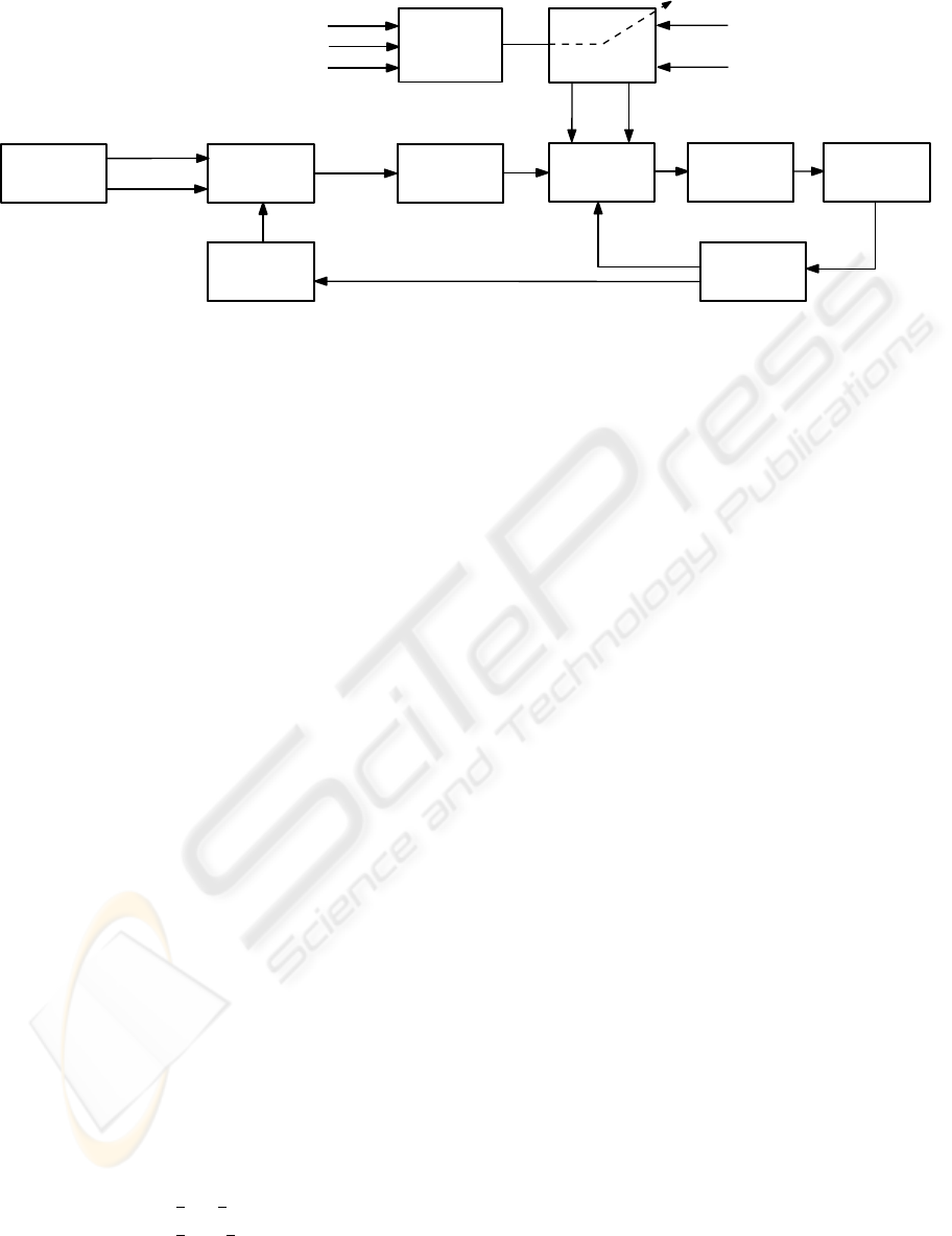
4.2 Control Design

The complete adaptive control system proposed in

this paper for the trajectory tracking of WMR is de-

picted in Figure 3. Some variables in this ﬁgure are

deﬁned later in the following paragraphs. At this

point one should particularly note the cascade ap-

proach which divides the control problem in two main

tasks namely, kinematic control and dynamic control.

The kinematic controller ensures that the robot tracks

a reference trajectory, which can be generated in real-

time (one time-step ahead) by a path-planning algo-

rithm. To achieve this the kinematic controller issues

a velocity command that serves as the reference signal

for the adaptive dynamic controller. The latter com-

putes a control torque by employing the estimated dy-

namic functions, obtained from the ANN stochastic

estimator, in order to ensure that the robot velocity

ICINCO 2006 - ROBOTICS AND AUTOMATION

408

Trajectory

generator

Velocity

converter

WMR

Dynamic

controller

Sample

& hold

order

hold

Kinematic

controller



k+1



k+1



k+1



k+1

Zero order

hold

ˆw

k+1

Stochastic

weight

tuner

ANN

function

estimator

k−1

Figure 3: Complete adaptive scheme.

vector really tracks the velocity desired by the kine-

matic controller. These two sub-controllers are de-

tailed next.

A very simple, yet useful representation of the tra-

jectory tracking problem, is through the concept of

the virtual vehicle (Crowley, 1989). Basically, the

time dependent trajectory to be tracked by the WMR

is designated by a non-stationary virtual vehicle hav-

ing the same nonholonomic constraints as the real

robot. The controller aims for the real vehicle to

track the virtual vehicle at all times, in both posture

and velocity. The discrete-time tracking error vector

= [e

]

is deﬁned as:





cos φ

sin φ

− sin φ

cos φ

0 0 1





− p

) , (29)

where p

= [x

]

denotes the virtual ve-

hicle sampled pose vector. In trajectory tracking the

aim is to make e converge to zero so that p converges

to p

. For this task we propose a discrete-time version

of the continuous-time kinematic controller originally

presented in (Kanayama et al., 1990) given by:



cos e

+ k

sin e



, (30)

where ν

is the wheel velocity command vector re-

quested by the kinematic controller, (k

, k

) > 0

are design parameters, and v

, ω

are the transla-

tional and angular velocities respectively correspond-

ing to the virtual vehicle. The latter are directly re-

lated to the virtual vehicle wheel velocity vector ν

as follows



−





. (31)

If we ignore the dynamic effects and consider only

the kinematic model (4) of the WMR and assume

perfect velocity tracking, then (30) completely solves

the trajectory tracking problem. However if a dy-

namic controller is to be implemented and assuming

no uncertainty in f

and G, one can use the following

dynamic control law to ensure that the WMR velocity

vector ν

really tracks ν

= f

+ G



k+1

− ν

+ k

{ν

− ν

}



, (32)

where −1 < k

< 1 is a design parameter. Note that

the control law requires the velocity command vec-

tor ν

to be known one sampling interval ahead. For

this reason we advance the kinematic control stage by

one sampling interval. This is achieved by: gener-

ating the reference trajectory vectors corresponding

to the (k + 1) instant, and using a ﬁrst order hold to

estimate p

k+1

from p

. The latter is a valid approx-

imation since any decent sampling rate (in the order

of milli seconds) is still high enough compared to the

relatively slow dynamics of a mobile robot. Substitut-

ing this control law in the stochastic dynamic model

in (10) yields the following closed loop dynamics:

k+1

= ν

k+1

+ k

(ν

− ν

) − ǫ

k+1

. (33)

Equation (33) clearly indicates that |ν

− ν

| → ǫ

as k → ∞. It is interesting to note that the case with

= 0, corresponds to the deadbeat control con-

cept associated with digital control systems. When

the dynamics are completely unknown and/or prone

to change, we propose to replace the control law (32)

with its heuristic certainty equivalent, utilising the es-

timates

and

from the ANN, leading to the

adaptive control law:



k+1

− ν

+ k

{ν

− ν

}



. (34)

NEURO-ADAPTIVE DYNAMIC CONTROL FOR TRAJECTORY TRACKING OF MOBILE ROBOTS

409

0 60 120 180

0.1

0.2

0.3

0.4

(a)

k p

− p k

−3 −2 −1 0 1 2 3

−4

−2

(b)

x (m)

y (m)

0 60 120 180

−20

(c)

Torque vector (Nm)

0 60 120 180

−10

(e)

Innovations vector i

time (s)

0 60 120 180

−1

(d)

v (m/s) & ω (rad/s)

0 60 120 180

100

(f )

time (s)

Diagonal mean of P

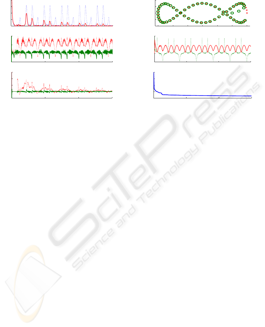
Figure 4: (a): adaptive (solid) & nonadaptive (dashed); (b): reference (×) & actual (◦) trajectories (ﬁrst 60 seconds); (c): right

wheel (dashed) & left wheel (solid) torques; (d): linear (solid) & angular (dashed) velocities; (e): innovations vector i

; (f):

diagonal mean of P

. Plots (b) to (f) correspond to the proposed adaptive controller.

5 SIMULATION RESULTS

The proposed neuro-adaptive dynamic controller

(34) was veriﬁed and compared to its non-

adaptive version (32) by highly realistic simula-

tions. The mobile robot was simulated through

the continuous-time, full kinematic/dynamic model

given in (4) and (6) with the following parame-

ters: b=0.5m, r=0.15m, d=0.2m, m

=30kg, m

=1kg,

=15.625kgm

, I

=0.005kgm

, I

=0.0025kgm

We included viscous friction by setting F ( ˙q) = F

˙q

in (7), where F

is a diagonal matrix of coefﬁcients

whose diagonal was set to [2, 2, 5, 0.5, 0.5]. Sampling

interval T = 50ms and the sampled data was cor-

rupted with noise ǫ

. To make the simulations more

realistic we imposed hard limits on the wheel torques

(±50Nm) to simulate actuator saturation. Neural net-

work pre-training is not used and to demonstrate fur-

ther the adaptive feature of the proposed controller,

the model used for simulations is abruptly modiﬁed

at t = 10s by introducing an additional load of 15kg

placed 0.4m away from P

. Moreover, at the same in-

stant we simulate a fault in the right wheel by increas-

ing its viscous friction coefﬁcient by a factor of ten.

The reference trajectory used for simulations is very

demanding since it is characterised by high velocities

and accelerations. The neural network contained 49

RBFs with covariance matrix R

= 100I

, where I

denotes an (i × i) identity matrix. The Kalman ﬁlter

initial covariance P

= 100I

, where α is the total

number of weights. The initial weight vector ˆw

was

generated from a normal distribution with zero mean.

It took a standard desktop computer with no code op-

timisation merely 1 minute to simulate 3 minutes of

real-time. Clearly, this indicates that the proposed al-

gorithm is not computationally demanding.

A number of results for this particular simulation

are presented in Figure 4. Plot (a) shows clearly the

difference in performance between the adaptive and

nonadaptive controllers. In both cases the Euclid-

ian vector norm of the pose error diminishes quickly

from some non-zero initial value. However from

t = 10s onwards, corresponding to the aforemen-

tioned model disruption, the adaptive controller reacts

to the change and after a transitional period manages

to reduce the pose error vector back to normal; the

ANN has adapted to the new dynamic functions. As

expected this does not happen in the nonadaptive case

and the pose error remains relatively higher ∀t > 10s.

The actual trajectory in the x y plane is superimposed

on the reference trajectory in plot (b), which also ver-

iﬁes the good tracking performance of the proposed

scheme. Plot (c) depicts the wheel torque vector τ

and in (d) one should particularly note the high val-

ues of the translational v and angular ω velocities of

the WMR. Plot (e) shows how the Kalman innovation

vector abruptly increases at 10s due to the model dis-

ruption and diminishes back with time as the ANN

weights adapt to the new situation. Plot (f) depicts the

mean of the diagonal of the covariance matrix P

time. The latter provides a measure of the uncertainty

in the estimated weights, as generated recursively by

the Kalman ﬁlter. As expected, the uncertainty de-

creases with time, indicating that the Kalman ﬁlter is

stable and the neural network estimations are contin-

uously improving. The slope of this curve is related

to the learning rate of the ANN adaptive scheme.

ICINCO 2006 - ROBOTICS AND AUTOMATION

410

6 CONCLUSIONS

In this paper an ANN functional-adaptive dynamic

control scheme for the trajectory tracking problem of

mobile robots is proposed. The resulting algorithm

requires no preliminary information about the nonlin-

ear functions in the dynamics and uses a RBF neural

network, trained online in consideration of noise, un-

certainty and disturbances by using a Kalman ﬁlter.

The designed scheme was tested successfully by real-

istic simulations for several noise conditions and pa-

rameter variations. The adaptive controller showed

improved performance when compared to the non-

adaptive case in the face of parameter uncertainty. Fu-

ture research will investigate the use of parameter re-

setting in the estimator and the development of dual

stochastic nonlinear control laws (Fabri and Kadirka-

manathan, 2001) which would take into account the

inaccuracy of the ANN approximations, giving rise to

better transient performance. We anticipate to get sat-

isfactory experimental results once the proposed al-

gorithm is implemented on a real mobile robot in the

near future.

REFERENCES

Brockett, R. W. (1983). Asymptotic Stability and Feedback

Stabilisation. Differential Geometric Control Theory.

Birkh

auser, Boston, MA.

Bugeja, M. K. and Fabri, S. G. (2005). Multilayer percep-

tron functional adaptive control for trajectory track-

ing of wheeled mobile robots. In Proc. 2nd Interna-

tional Conference on Informatics in Control, Automa-

tion and Robotics (ICINCO2005), volume 3, pages

66–72, Barcelona, Spain.

Canudas de Wit, C., Khennoul, H., Samson, C., and Sor-

dalen, O. J. (1993). Nonlinear control design for mo-

bile robots. In Zheng, Y. F., editor, Recent Trends

in Mobile Robots, Robotics and Automated Systems,

chapter 5, pages 121–156. World Scientiﬁc.

Corradini, M. L., Ippoliti, G., and Longhi, S. (2003). Neural

networks based control of mobile robots: Develop-

ment and experimental validation. Journal of Robotic

Systems, 20(10):587–600.

Corradini, M. L. and Orlando, G. (2001). Robust tracking

control of mobile robots in the presence of uncertain-

ties in the dynamic model. Journal of Robotic Sys-

tems, 18(6):317–323.

Crowley, J. L. (1989). Asynchronous control of orienta-

tion and displacement in a robot vehicle. In Proc. of

the 1989 IEEE International Conference on Robotics

and Automation (Vol. 3), pages 1277–1282, Scotts-

dale, AZ.

de Sousa, C., Hemerly, E. M., and Galvao, R. K. H. (2002).

Adaptive control for mobile robot using wavelet net-

works. IEEE Transactions on Systems, Man and Cy-

bernetics, 32(4):493–504.

Ding, D. and Cooper, R. A. (2005). Electric-powered

wheelchairs. IEEE Control Systems Magazine,

25(2):22–34.

Fabri, S. G. and Kadirkamanathan, V. (1998). Dual adaptive

control of nonlinear stochastic systems using neural

networks. Automatica, 34(2):245–253.

Fabri, S. G. and Kadirkamanathan, V. (2001). Functional

Adaptive Control: An Intelligent Systems Approach.

Springer-Verlag, London, UK.

Fierro, R. and Lewis, F. L. (1995). Control of a nonholo-

nomic mobile robot: Backstepping kinematics into

dynamics. In Proc. IEEE 34th Conference on Deci-

sion and Control (CDC’95), pages 3805–3810, New

Orleans, LA.

Fierro, R. and Lewis, F. L. (1998). Control of a non-

holonomic mobile robot using neural networks. IEEE

Trans. Neural Networks, 9(4):589–600.

Fukao, T., Nakagawa, H., and Adachi, N. (2000). Adap-

tive tracking control of a nonholonomic mobile ro-

bot. IEEE Transactions on Robotics and Automation,

16(5):609–615.

Kalman, R. E. (1960). A new approach to linear ﬁltering

and prediction problems. Trans. ASME J. Basic Eng.,

82:34–45.

Kanayama, Y., Kimura, Y., Miyazaki, F., and Noguchi, T.

(1990). A stable tracking control method for an au-

tonomous mobile robot. In Proc. IEEE International

Conference of Robotics and Automation, pages 384–

389, Cincinnati, OH.

Kolmanovsky, I. and McClamroch, N. H. (1995). Develop-

ments in nonholonomic control problems. IEEE Con-

trol Systems Magazine, 15(6):20–36.

Lamiraux, F., Laumond, J. P., VanGeem, C., Boutonnet,

D., and Raust, G. (2005). Trailer truck trajectory op-

timization: the transportation of components for the

Airbus A380. IEEE Robotics and Automation Maga-

zine, 12(1):14–21.

Maybeck, P. S. (1979). Stochastic Models, Estimation and

Control, volume 141-1 of Mathematics in Science and

Engineering. Academic Press Inc., London, UK.

Oubbati, M., Schanz, M., and Levi, P. (2005). Kinematic

and dynamic adaptive control of a nonholonomic mo-

bile robot using RNN. In Proc. IEEE Symposium on

Computational Intelligence in Robotics and Automa-

tion (CIRA’05), Helsinki, Finland.

Poggio, T. and Girosi, F. (1990). Networks for approxima-

tion and learning. Proc. IEEE, 78(9):1481–1497.

Sarkar, N., Yun, X., and Kumar, V. (1994). Control of

mechanical systems with rolling constraints: Appli-

cations to dynamic control of mobile robots. Interna-

tional Journal of Robotics Research, 13(1):55–69.

van de Water, H. and Willems, J. C. (1981). The cer-

tainty equivalence property in stochastic control the-

ory. IEEE Transactions on Automatic Control, AC-

26(5):1080–1087.

NEURO-ADAPTIVE DYNAMIC CONTROL FOR TRAJECTORY TRACKING OF MOBILE ROBOTS

411