
A PERFORMANCE METRIC FOR MOBILE ROBOT
LOCALIZATION
Antonio Ruiz-Mayor, Gracián Triviño, Gonzalo Bailador
Depto. Tecnología Fotónica, Universidad Politécnica de Madrid, Campus de Montegancedo s/n, Boadilla del Monte, Spain
Keywords: Robot localization, pose estimation, performance metric, benchmark, prediction-correction.
Abstract: This paper focus on the problem of how to measure in a reproducible way the localization precision of a
mobile robot. In particular localization algorithms that match the classic prediction-correction model are
considered. We propose a performance metric based on the formalization of the error sources that affect the
pose estimation error. Performance results of a localization algorithm for a real mobile robot are presented.
This metric fulfils at the same time the following properties: 1) to effectively measure the estimation error
of a pose estimation algorithm, 2) to be reproducible, 3) to clearly separate the contribution of the correction
part from the prediction part of the algorithm, and 4) to make easy the algorithm performance analysis
respect to the great number of influencing factors. The proposed metric allows the validation and evaluation
of a localization algorithm in a systematic and standard way, reducing workload and design time.
1 INTRODUCTION
Experimentation in Autonomous Mobile Robots
(AMR) research is not an obvious task. This type of
robots are complex systems. They incorporate a
great number of interrelated hardware and software
subsystems. Their navigation environment must be
specifically modelled and their components must
operate in real time. Finally, any research
contribution about autonomous behaviours in real
environments requires a considerable effort in both
theoretical and experimental works.
Performance evaluation for such complex
systems is likewise a complex task. Experiments
must be controlled and reproducible, but it is not
easy to repeat the experiments of another research
group because of the high number of involved
variables. There exist an important need to establish
general frameworks of performance evaluation, in
the context of intelligent systems (Meystel et al,
2003) and more specifically about AMRs (Dillman,
2004). The work of (Hanks et al, 1993) goes ahead
and remarks the need of benchmarks that not only
provide performance comparisons, but that also
support the scientific progress by helping to analyze
why the system behaves the way it does.
Furthermore, the development of this area will be a
requirement for AMR systems to reach the consumer
market.
A main feature for robot autonomy is the self-
localization capability. The robot must estimate by
itself its pose (position and orientation) respect to a
reference system, with enough precision to achieve
the commended tasks. The particular problem we
focus is how to measure in a reproducible way the
precision of the pose estimations produced by the
robot. The solution of this problem will allow the
validation and performance evaluation of a
localization algorithm in a systematic and standard
way, reducing design time and workload.
Our hypothesis is that it is possible to perform
systematic and reproducible measurements of the
pose estimation error in real navigation conditions.
Although there are a great number of influencing
factors, we believe that they can be enumerated and
modelled. In section 2 we formalize the pose
estimation process, In section 3, a reproducible
performance metric for robot localization is
proposed. Experimental results are presented and
discussed in section 4, followed by the main
conclusions in section 5.
This work has been supported by the project
Precompetitivo UPM 14120 "Sancho 3. Diseño y
construcción de un robot móvil de propósito general".
269
Ruiz-Mayor A., Triviño G. and Bailador G. (2006).
A PERFORMANCE METRIC FOR MOBILE ROBOT LOCALIZATION.
In Proceedings of the Third International Conference on Informatics in Control, Automation and Robotics, pages 269-276
DOI: 10.5220/0001218602690276
Copyright
c
SciTePress
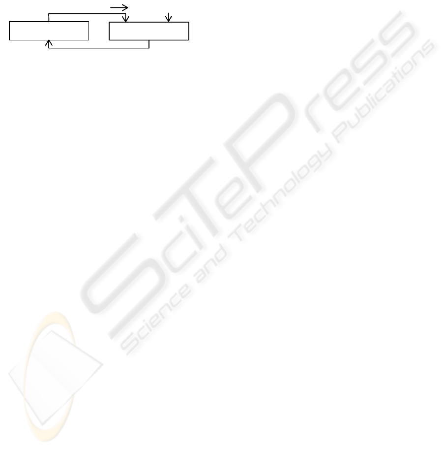
2 THE PREDICTION-
CORRECTION MODEL
Most solutions to AMR pose estimation follow the
classic prediction-correction (or predict-update)
closed loop state estimator model presented in
Figure 1. According to (Thrun, 2002), virtually all
state of the art robotic mapping algorithms are
probabilistic, and the single dominating scheme for
state estimation is the Bayes filter, a recursive
estimator that matches the prediction-correction
model. A particular bayesian filter of common use in
AMR localization is the Kalman Filter (Welch and
Bishop, 2004). But other non-probabilistic solutions
also follow this model, for example the possibilistic
approach of (Bloch and Saffioti, 2002). This
widespread and simple scheme estimates the robot’s
pose in two steps: prediction and correction. The
prediction is achieved by an algorithm (AP in
advance) that implements the process model:
),
ˆ
(
ˆ
1
kk
k
uxAx =
+
−
(2-1)
where
k
x
ˆ
is the estimation of the robot’s state at step
k,
k
u is the control action that was ordered at step k
to reach the step k+1, A is the process model, and
1
ˆ
+
−
k
x is the a priori estimation of the robot’s state at
step k+1.
k
x
ˆ
must contain the robot’s pose, that is
habitually in the form of a vector composed by two
cartesian position coordinates and one orientation
coordinate respect to a reference system external to
the robot. In an AMR system the process model A
often represents a fine tuned dead-reckoning model
for the actual motor robot platform. It includes
physical wheels dimensions, odometers resolution,
models of the motor control algorithms, etc.
If the pose is estimated in open loop using only
the AP, the estimation error in
1
ˆ
+
−
k
x increase
monotonically along the trajectory and the robot will
be lost or will collide. The classic solution to this
problem is using exteroceptive sensors like sonar,
laser, CCD cameras, etc. to capture some actual
perception z
k
of the surrounding objects and
comparing it against a map of the environment. Here
begins the algorithm of the correction phase (in
advance, AC), that fuses the a priori estimation with
the information that comes from
k
z to obtain the
posterior state estimation
k
x
ˆ
. The correction
estimator function E is expressed as:
))
ˆ
(,,
ˆ
(
ˆ
k
k
k
k
xHzxEx
−−
= (2-2)
where H(x
i
) models the robot’s perception at a
particular state x
i
. It must include the sensor model
and the measurement model involved in the capture
of
k
z .The estimator E must correct the a priori
estimation by comparing the actual perception
k
z
with H(
k
x
−
ˆ
), the expected perception at
k
x
−
ˆ
. Every
variable in this loop has an associated uncertainty,
that have not been represented in the previous
equations for simplicity. E may use the uncertainties
of
k
x
−
ˆ
,
k
z and the uncertainty derived from the
comparison of
k
z with H(
k
x
−
ˆ
) to perform the states
fusion.
2.1 Estimation Error Evaluation
The AP-AC tandem conforms an algorithm for the
estimation of the robot’s pose (in advance, AEP). Its
performance is typically evaluated by the error of
the estimated pose (in advance, EEP) respect to the
real pose. The particular operators that compute the
EEP will be presented in the next section.
Note that the EEP may be applied to both
k
x
−
ˆ
and
k
x
ˆ
estimations. The AC is responsible of the
final estimation and, apparently, is the key of the
process, but, how much effective is the AC respect
to the AP? Suppose a robot with good quality
odometers an a fine tuned AP (easy to build
nowadays), precise enough to keep
k
x
−
ˆ
below the
application location error requirements along several
meters of trajectory. In most cases the AC will be
just copying
k
x
−
ˆ
to
k
x
ˆ
, but having to compute the
code from H and E functions. A common situation is
to find that AC (world model, sensor model, etc)
complexity is much greater than the one of the AP. It
is worth in such cases to spend a great deal of
computation in the AC? How the computational load
between the AP and the AC can be balanced without
degrading the AEP performance? We propose to
analyze the posterior estimation error relative to the
a priori error as one of the key elements that may
help to explain the performance of an AEP in terms
of its internal components. This approach is one step
ahead from the obtaining of a simple performance
metric punctuation, in the sense of the (Hanks et al,
1993) reference in section 1, and is the main part of
the performance metric presented in section 3.
Figure 1: The generic prediction-correction model.
x
k
^
x
-
k+1
^
(k+1 k)
z
k
Prediction (AP)
Correction (AC)
x
k
^
x
k
^
x
-
k+1
^
x
-
k+1
^
(k+1 k)
z
k
Prediction (AP)
Correction (AC)
ICINCO 2006 - ROBOTICS AND AUTOMATION
270

Nowadays, there is no a widely accepted
performance metric for measuring in a reproducible
way the localization precision of a mobile robot.
Furthermore, there are few published works that
propose performance metrics for robot localization.
In (O’Sullivan et al, 2004) an interesting
performance metric for map building is presented.
Although the pose estimation is intimately involved
in the map building task, this metric does not
separate the performance of the pose estimation
from the world modelling algorithms. (Gat, 1995)
emphasizes on the experiments reproducibility and
propose a performance metric for AMRs that
measures the traversed distance and elapsed time to
reach a goal. Here again the pose estimation
performance is enclosed with another robot’s
subsystems. In the general robot localization
literature, a very common way to evaluate the EEP
is to measure quantitatively the position and
orientation error, see for example (Lee and Song,
2004) and (Clerentin et al, 2005). Other works do
not measure quantitatively the EEP, as (Sagüés and
Guerrero, 2005) which controls the EEP by making
the robot to stop periodically in a checkpoint marked
on the floor and counting the times it does inside the
marks. Some works, such as (Porta et al, 2005),
report in detail the experiments conditions. Others,
like (Castellanos et al, 2001), also report the
statistical significance of the obtained EEP
distributions. But only few works as (Fox et al,
1999), (Gutmann and Fox, 2002) and (Di Marco et
al, 2004) present experimental results with enough
quality and detail to match the requirements of a
performance metric. Experiments conditions are also
reported as exhaustively to be reproduced. In such
cases, the pose estimation error is reported as a
whole, without analysing the AC contribution to the
final EEP, as exposed as follows.
3 PERFORMANCE METRIC
We propose a performance metric for benchmarking
the correction algorithm AC based on formalizing
the error sources to prevent hidden factors that could
falsify the obtained EEP. The metric is composed by
the following steps:
1. Experiments framework report
2. Run conditions report
3. Analysis of the absolute estimation error
4. Analysis of the estimation error relative to the
a priori error
Steps 1 and 2 are a collection of requirements to
describe the navigation experiments (runs) with
enough detail to be reproducible. Steps 3 and 4 are
the metric itself. The term “run” is used here as a
controlled experiment in which the robot travels
along a monitorized trajectory. The AEP developer
should decide the rooms and trajectories depending
on his/her research objectives. During every run, the
trajectory’s real poses x
i
should be sampled with
enough frequency to obtain representative statistical
distributions. This sampling should be done using
measurement instruments external to the robot and
its precision, the ground truth of the experiment,
should be at least twice the AEP’s expected
precision. The robot should record the a priori and
posterior estimations produced for each sampled real
pose. In consequence for every run i three traces of
poses should be obtained:
}
ˆ
...
ˆ
,
ˆ
{
}
ˆ
...
ˆ
,
ˆ
{
}...,{
21
21
21
Ni
i
Nii
Nii
xxxPEprio
xxxPEpost
xxxRP
−−−
=
=
=
(3-1)
where RP
i
, PEpost
i
, and PEprio
i
are the traces of
real poses, posterior pose estimations and a priori
pose estimations from the run i, respectively. N
i
is
the number of sampled real poses in the run i, and i
= 1..R, being R the number of runs. Metric
components are explained in the following sections.
3.1 Experiments Framework Report
In order to document the EEP factors with sufficient
detail, the AEP developer should first describe the
general experiments framework, common to every
run. It should be reported the general objectives of
the particular AEP development, the type of AMR
(general or specific purpose, etc), the type of
navigation environment (indoor, outdoor, office,
domestic, industrial, etc.), and how these aspects
condition the run selection.
The AC should be documented in terms of the
description of the E and H functions and their
uncertainty models. Additionally, it should be
reported as exhaustively as possible the frequency of
the AC estimations: respect to the AP estimation
frequency, to the absolute time, to the robot travelled
distance, etc. The procedure and frequency of real
poses measurement, and its ground truth should also
be reported. In the case of simulated runs, it should
be described the simulator internal models.
3.2 Run Conditions Report
This report must contain the experiment features that
may change between runs. For each run, the place
where it has been performed should be described. At
A PERFORMANCE METRIC FOR MOBILE ROBOT LOCALIZATION
271

least the walls and obstacles topology, their material
properties and the ambient conditions should be
presented. It should also be described any other
factor that may affect the capture of the robot
exteroceptive sensors. Additionally, the run
trajectory should be included, at least the RP
i
,
PEpost
i
, and PEprio
i
traces and (i = 1..R). A
graphical 2D floor projection is a conventional way
to present the trajectories. The criteria for
trajectories generation should be reported.
It should be justified why each run is
representative of real trajectories and how the
statistical parameters derived from it are valid, in
terms of sufficient number of samples, use of
random or controlled trajectories, etc. The eventual
environment changes during the run should be
quantified, to describe the degree in which the run
represents dynamic environments, for example,
number of perceptible people during the run, etc.
3.3 Analysis of the Absolute
Estimation Error
The objective of this analysis is the absolute AEP’s
performance in terms of position and orientation
errors of the captured posterior estimations PEpost
i
.
Lets first define the EEP as a set of a position error
EEP
XY
and an orientation error EEP
T
:
),
ˆ
()
ˆ
(
),
ˆ
()
ˆ
(
iiTiT
iiXYiXY
xxdxEEP
xxdxEEP
=
=
(3-2)
where x
i
is the real pose measured under
controlled conditions when the robot produced the
estimation
i
x
ˆ
, d
XY
is the euclidean distance between
positions over the plane of the floor, and d
T
is the
absolute orientations angle difference (euclidean
distance over the orientation dimension). We chose
euclidean distances because they are intuitive and of
common use. For example, the requirements of an
AEP development project can be expressed as “The
95% of the EEP should be under 20cm, 5º.”
Distributions of the posterior EEP
XY
and EEP
T
for
the run i (i = 1..R) are defined as:
}
ˆ
/)
ˆ
({
}
ˆ
/)
ˆ
({
ijjTi
ijjXYi
PEpostxxEEPEEPpostT
PEpostxxEEPEEPpostXY
∈=
∈=
(3-3)
The data of interest are the R bidimensional
distributions EEPpostXY
i
vs. EEPpostT
i
. The
distributions should be analysed in terms of the
following parameters:
-
Ground truth limits: Every distribution point
should be above the ground truth.
-
Relevant percentiles: 100%, 95%, 90%, etc.
They allow runs comparisons in terms of
position and orientation precision.
-
(If available) The theoretical limit of the
optimal AEP performance. It lets to analyze
what percentage of estimations are optimal.
Observed differences between run distributions
should be explained in terms of the run conditions
factors presented in the previous section. If the
differences are well explained and the runs are
representative of the robot’s target navigation
environment, the union of all distributions may be
analyzed as a single bidimensional distribution to
represent the global AEP performance metric.
3.4 Analysis of the Estimation Error
Relative to the a Priori Error
This analysis focus on the AC performance. The
objective is to measure the AC capability to
effectively reduce the EEP, independently from the
AP efficiency. The distributions of the a priori
EEP
XY
and EEP
T
for the run i (i = 1.. R) are defined
as:
}
ˆ
/)
ˆ
({
}
ˆ
/)
ˆ
({
ijjTi
ijjXYi
PEprioxxEEPEEPprioT
PEprioxxEEPEEPprioXY
∈=
∈=
(3-4)
The data to be analyzed are the R bidimensional
distributions EEPpostXY
i
vs. EEPprioXY
i
(EEP
XY
analysis) and the R bidimensional distributions
EEPpostT
i
vs. EEPprioT
i
(EEP
T
analysis). Both data
sets will be analyzed in the following way: 1) For
every run, Quantify in a factor C
XY
the percentage of
estimations
j
x
ˆ
that improve the EEP
XY
:
)
ˆ
()
ˆ
(
j
XYjXY
xEEPxEEP
−
≤ (3-5)
2) Quantify in a factor C
T
the same percentage for
EEP
T
:
)
ˆ
()
ˆ
(
j
TjT
xEEPxEEP
−
≤ (3-6)
3) Quantify in a factor C
XYT
the same percentage
that holds (3-5) and (3-6) at the same time.
C
XY
, C
T
and C
XYT
factors represent the AC
capability to really correct the EEP under the
navigation conditions of the runs set.
In the same way as the previous analysis, the
differences between run distributions should be
explained in terms of the run conditions factors. If
the differences are well explained and the runs are
representative of the robot’s target navigation
environment, the union of all distributions may be
analyzed as a single bidimensional distribution to
represent the global AC performance metric.
ICINCO 2006 - ROBOTICS AND AUTOMATION
272
The analysis may be extended by the addition of
other elements, like the injection of noise to
k
x
−
ˆ
to
increase the dynamic range of the a priori EEP. This
range may be interpreted as the degradation level of
the error sources that affect the AP. We can study
the portion of any posterior EEP distribution in a
particular interval of the a priori EEP range, and
quantify how the posterior EEP distribution will be
consequently affected. Additionally, the degradation
of error sources that affect the another AC input, the
z
k
perception, may be represented by designing
various run experiments with different levels of
perception noise.
4 EXPERIMENTAL RESULTS
The proposed performance metric has been applied
to a particular AEP developed by the authors. The
four metric steps are presented in next sections.
4.1 Experiments Framework Report
The target AEP is being developed in the frame of a
research project which main objective is the design
robotic platforms and tools for helping the AMR
research groups. The aim of this AEP development
is to implement a simple self-localization module
that validate the robot subsystems by showing
autonomous navigation in indoor office
environments.
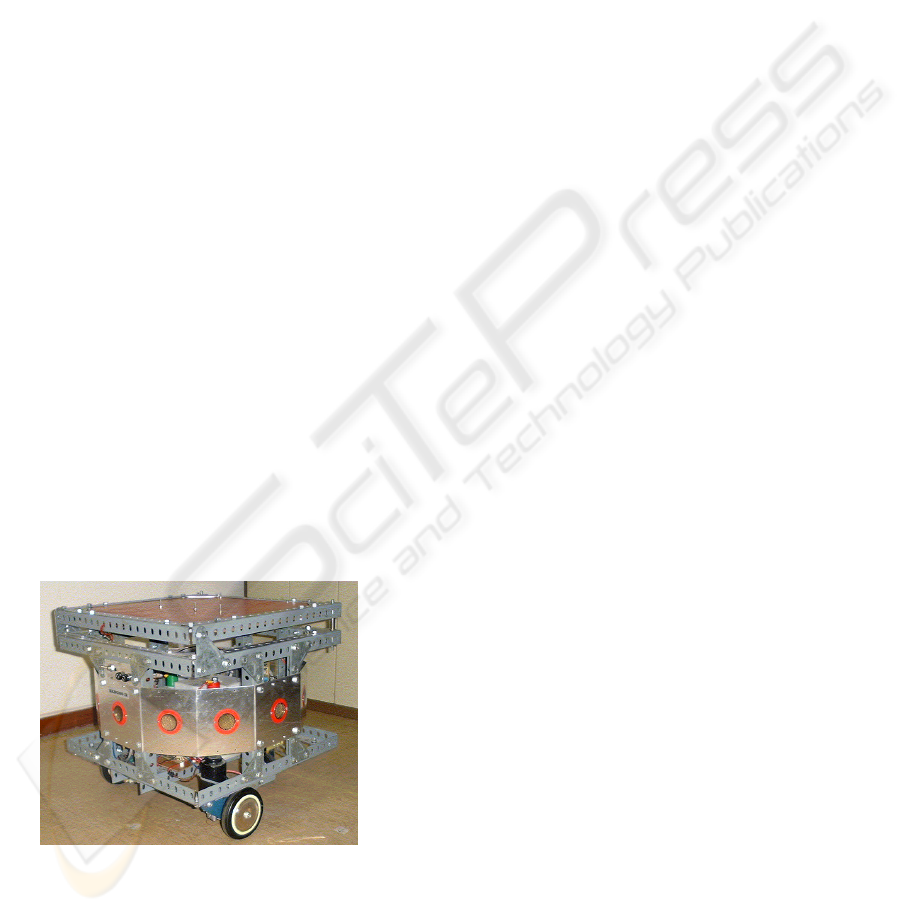
The robotic platform used is Sancho-2 (see
Figure 2), a mobile robot completely designed and
built by the authors for research purposes. Its
dimensions are 50cm wide, 50cm long and 50cm
high, that contains the hardware of the motors and
sensors control subsystems. High level software
components are implemented in a laptop PC that is
placed on the upper tray and connected by a serial
cable. The wheels have a tricycle structure, with two
motorized wheels and one castor wheel. The
resolution of the odometric sensors is 1.2cm. The
environment perception are achieved by a ring of
twelve ultrasonic sensors, whose resolution is 4cm.
Our AEP is an appearance-based approach and
works as follows: Once the AP has produced the a
priori estimation
k
x
−
ˆ
, a complete sonar capture is
fired. It produces a 12 echoes vector (z
k
) that may
be interpreted as a point in a 12 dimensions vectorial
space. The AC correction estimator E is expressed
as:
))(,((
ˆ
1
LPknnk
GHzfHx
−
= (4-1)
The expected perception is modelled as a points
cloud in the perception space by the following way:
A grid G
LP
of local poses x
i
is generated around the a
priori pose estimation
k
x
−
ˆ
, and for each of them its
expected perception H(
i
x ) is computed. The
parameters of G
LP
are the position and orientation
grid steps, s
XY
= 10cm and s
T
= 10º, and the grid radii
from its centre, 40cm, 40º. These values determine
the theoretical maximum EEP that our AC can
correct.
The H function models the robot environment as
a previously given map where the walls and
obstacles are represented by a set of 2D line
segments. The function returns, for each particular
ultrasonic sensor pose, the distance to the nearest
line segment inside a sensor cone with an aperture
angle of 30º. It does not calculate any kind of sonar
rebounds or outliers. This model is also used to
emulate the robot’s perception in the simulation
tests.
The actual perception z
k
is matched against the
expected perception cloud using the f
nn
function that
computes the nearest neighbour with the euclidean
distance. The posterior estimation
k
x
ˆ
is obtained by
the H
-1
function, by the identification of the grid
pose that produced the nearest perception.
As G
LP
is a discrete regular grid, the optimal
estimation respect to the EEP
XY
or EEP
T
metric is
obtained when the posterior estimation
k
x
ˆ
is also the
nearest neighbour in the positions plane or
orientations axis, respectively. To formalize this
concept we define the maximum reachable
precisions MPAxy (cm) and MPAt (º) parameters to
be the worst EEP
XY
or EEP
T
metric values that an
optimal estimation may obtain. It is easy to see that
MPAxy = 0.71 s
XY
, and MPAt = 0.5 s
T
. These
parameters will be needed in the section 4.3 and
their values for the experiments are 7.1cm and 5º.
The AP and AC estimation frequencies are equal
Figure 2: The mobile robot Sancho-2.
A PERFORMANCE METRIC FOR MOBILE ROBOT LOCALIZATION
273
and their value is 1 estimation per each 50cm
navigated. In this project’s phase, the runs have been
simulated. So, real pose measurement is exact and
its frequency may be the same as the one for AC
estimations, and the consequent ground truth is
0.0cm and 0.0º.
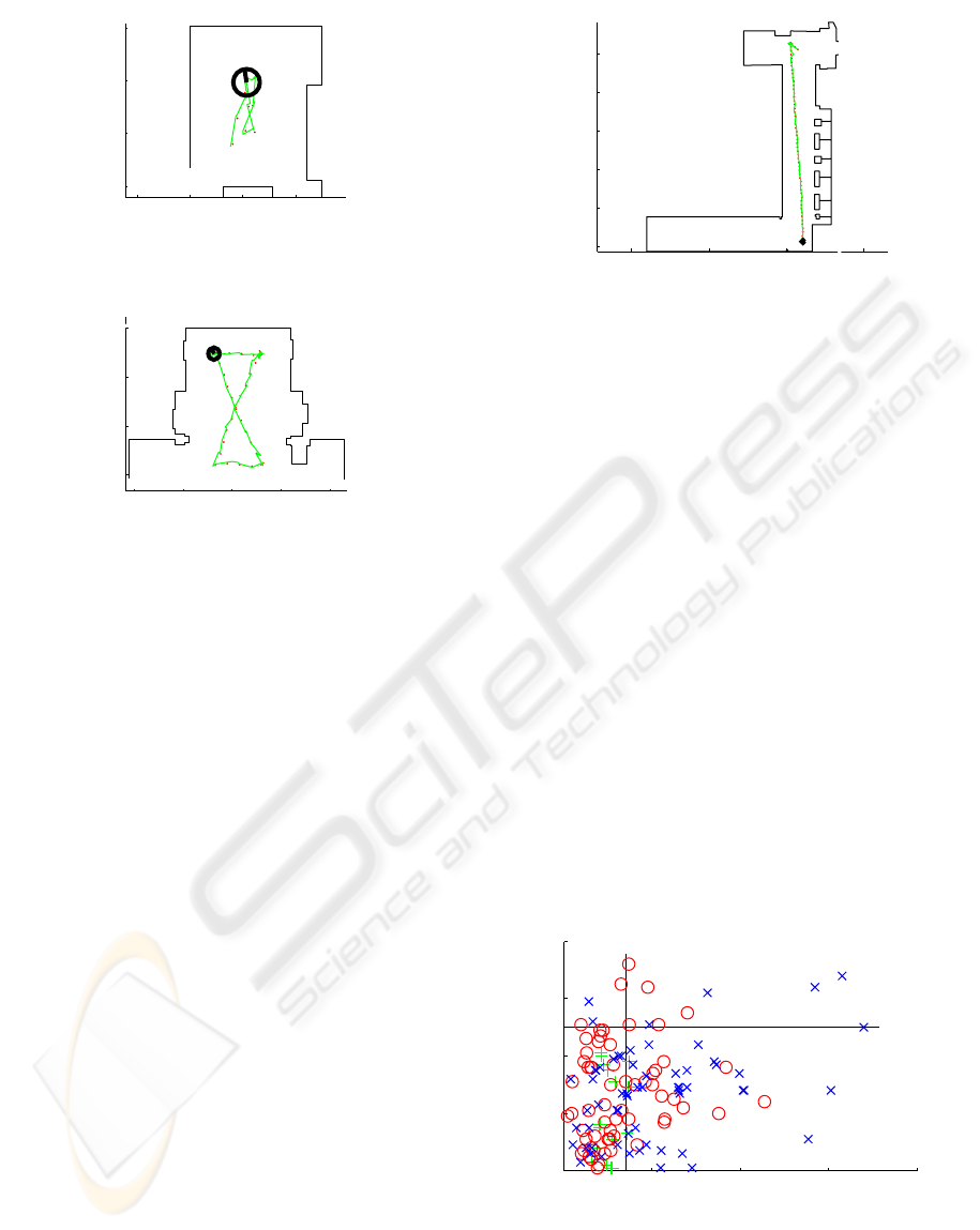
4.2 Run Conditions Report
Figures 3, 4 and 5 show the walls topology and
trajectories of the three runs, respectively. We have
selected real places from our Faculty buildings with
different areas and walls topologies to represent the
indoor navigation environments in an typical office
building. The navigation areas are small (2m
2
, R1),
medium (13m
2
, R2), and big (81m
2
, R3), and the
walls topologies are square (R1), open square (R2),
and corridor (R3). Every wall segment has been
modelled as having the same acoustic properties.
Regarding to the ambient conditions, we have
considered the room air temperature as a factor that
may change the sound speed and influence the
ultrasonic sensor precision. In our experiments this
temperature was 25ºC. The runs do not include
neither moving objects nor furniture changes.
To determine the trajectories, we have adopted
the criteria of travelling over most of the navigation
area and preventing trajectories coincidences. In the
corridor R3 the trajectory has been planned to
diagonally traverse only one time the place. In the
places R1 and R2 the trajectory draws an “8” over
the floor, passing by the four extremes of an
imaginary navigation rectangle. The runs produced
18 (R1), 62 (R2) and 61 (R3) estimations, resulting
in a total of 141 estimations. We did not increment
the R1 estimations to prevent the distribution slant
because this place is small and its punctuations are
better than the other ones.
Our AP a priori EEP distributions are upper-
bounded by the limits of 10cm and 5º. To full
characterize the AC response, we have injected to
the a priori estimation
k
x
−
ˆ
an uniform noise
distribution of which ranges are the theoretical limits
of our AC, the grid radii (40cm, 40º).
4.3 Analysis of the Absolute
Estimation Error
Figure 6 shows the three run distributions, under the
described experimentation conditions, including the
uniform noise injection to
k
x
−
ˆ
. Each run distribution
is represented with a different icon (see also Figure
7). Vertical and horizontal lines show the MPAxy
and MPAt limits, respectively (see section 4.1).
Figure 4: The run R2.
−200 0 200 400 600
−600
−400
−200
0
Y (cm)
X (cm)
Figure 5: The run R3.
−2000 −1000 0 1000
0
500
1000
1500
2000
2500
Y (cm)
X (cm)
Figure 3: The run R1.
−100 0 100 200
0
100
200
300
Y (cm)
X (cm)
Figure 6: Absolute estimation error distributions.
0 10 20 30 40
0
2
4
6
8
EEPpost (XY) (cm)
EEPpost (T) (º)
ICINCO 2006 - ROBOTICS AND AUTOMATION
274
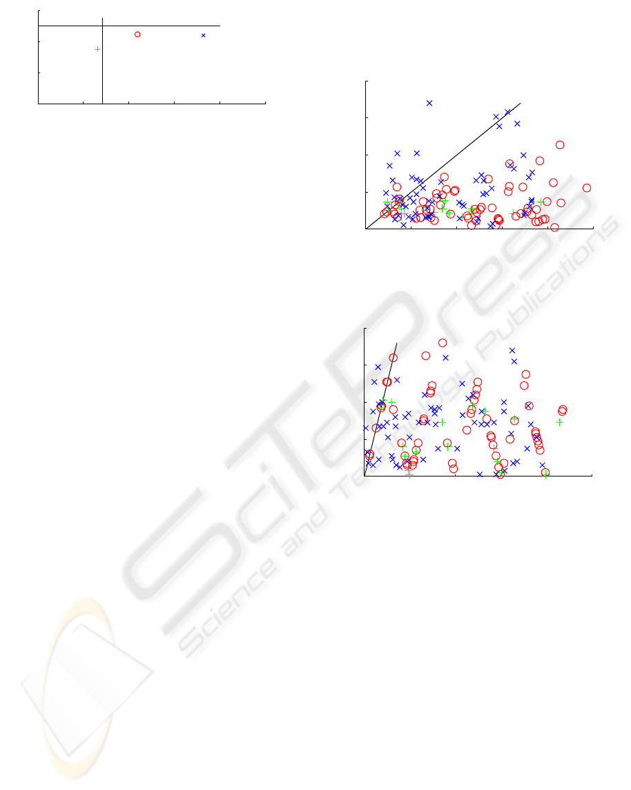
In order to explain the runs differences, Figure 7
reduces each run distribution to one point whose
coordinates are the the merit factors mfxy
i
and mft
i
:
iii
iii
ttmft
xyxymfxy
σμ
σμ
+=
+=
(4-2)
where μxy
i
and μt
i
are the means of EEPpostXY
i
and EEPpostT
i
, respectively, and σxy
i
and σt
i
are the
standard deviations of EEPpostXY
i
and EEPpostT
i
,
respectively. We explain the differences between the
3 runs by the size and walls disposition of the place
R1, the best result, is a small room and R3, the
worst, is a corridor.
Every punctuation is over the ground truth
(0.0cm, 0.0º). The maximum errors are 34.0cm and
7.2º that fall to 20.4cm, 5.7º at the 95% percentiles.
The percentage of optimal estimations, i.e. inside
both MPAxy and MPAt limits, are 53.2%.
The AEP show better performance in orientation
than in position estimation. If the final robot
application may accept a small orientation error
degradation, we could increase the s
T
grid parameter
to reduce the poses number of G
LP
, and consequently
reducing the computational cost of our AC.
4.4 Analysis of the Estimation Error
Relative to the a Priori Error
Figure 8 compares the posterior EEP
XY
vs. a priori
EEP
XY
distributions. Figure 9 shows the same
comparison in terms of the orientation error EEP
T
.
The line in the figures shows the limit where the
posterior EEP is equal to the a priori EEP. The
correction factors of our AEP are C
XY
= 88%, C
T
=
95% and C
XYT
= 84%. In future experiments we plan
to perform runs for producing a controlled
perception degradation.
4.5 Discussion
Performance metrics should measure the parameter
of interest, the measurement precision should be
enough and the metric process should be
reproducible. The proposed procedure may
effectively measure the interest parameter, the AC
estimation error, independently from the particular
AP to be used and other components performance,
through the noise injection to the a priori estimation
k
x
−
ˆ
. It has been shown that it is adequate to
measure it in two ways: absolute and relative to the a
priori error. It also has been shown that it is adequate
to make this measurement in the form of a set of
distributions instead of a single distribution or
numeric value, because each run distribution may be
affected by different factors from each others.
The sufficient metric precision is justified by the
requirement to the AEP developer to measure and
report the ground truth of the real pose measurement
process.
The metric reproducibility is guaranteed by the
high detail of the run conditions report and the runs
separation requirement. A run may be easily
reproduced using the report’s information. This is
also a tool for experiment validation.
This metric allows a great number of useful
performance comparisons. Different run
Figure 9: Relative orientation error distributions.
0 10 20 30 40 50
0
2
4
6
8
EEPprio (T) (º)
EEPpost (T) (º)
Figure 8: Relative position error distributions.
0 10 20 30 40 50
0
10
20
30
40
EEPprio (XY) (cm)
EEPpost (XY) (cm)
Figure 7: Absolute runs merit factor.
0 5 10 15 20 25
0
2
4
6
R1
R2
R3
EEPpost (XY) (cm)
EEPpost (T) (º)
A PERFORMANCE METRIC FOR MOBILE ROBOT LOCALIZATION
275

distributions may represent different run places,
robot platforms (APs), AEPs, temperature or
illumination conditions, trajectories in the same
room, etc.
5 CONCLUSION
The proposed performance metric offers a
contribution to the area of the mobile robotics
performance measurement, in particular in the robot
localization field. This metric differs from the works
found in the literature in the fact that it fulfils at the
same time the useful properties of 1) to effectively
measure the estimation error of a pose estimation
algorithm, 2) to be reproducible, 3) to clearly
separate the contribution of the correction algorithm,
and 4) to make easy the analysis of the algorithm
performance respect to the great number of
influencing factors.
REFERENCES
Bloch, I. and Saffiotti, A., (2002), Why Robots should use
Fuzzy Mathematical Morphology, Proc. 1st Int. ICSC-
NAISO Congress on Neuro-Fuzzy Technologies, La
Havana, Cuba, January 2002. Retrieved may, 2006
from http://www.aass.oru.se/~asaffio.
Castellanos, J.A., Neira, J., and Tardós, J.D., (2001),
Multisensor Fusion for Simultaneous Localization and
Map Building, IEEE Transactions on Robotics and
Automation, vol 17, no. 6, pp 908-914, dec. 2001.
Clerentin, A., Delahoche, L., Brassart, E., Drocourt, C.,
(2005), Self localization: a new uncertainty
propagation architecture, Robotics and Autonomous
Systems 51 (2005) 151-166, Elsevier.
Dillman, R., (2004), KA 1.10 Benchmarks for Robotics
Research, Technical Report from EURON IST-2000-
26048 European Robotics Research Network, pp 1-
21. 24th April 2004. Retrieved May, 2005, from
http://www.cas.kth.se/euron/euron-deliverables/ka1-
10-benchmarking.pdf
Di Marco, M., Garulli, A., Giannitrapani, A., and Vicino,
A., (2004), A Set Theoretic Approach to Dynamic
Robot Localization and Mapping, Autonomous Robots
16, 23-47, Kluwer Academic Publishers, 2004.
Fox, D., Burgard, W., Dellaert, F., and Thrun, S., (1999),
Monte Carlo Localization: Efficient Position
Estimation for Mobile Robots, Proc. 16th National
Conf. on Artificial Intelligence (AAAI-99), pp 343-
349, Orlando, Florida, 1999.
Gat, E., (1995), Towards principled experimental study of
autonomous mobile robots, Autonomous Robots, vol 2
num 3, pp 179-189, Springer, 1995.
Gutmann, J.S., and Fox, D., (2002), An Experimental
Comparison of Localization Methods Continued,
Proc. IEEE/RSJ Int. Conf. on Intelligent Robots and
Systems, IROS’02, vol I, pp454-9, Piscataway NJ,
USA, 2002.
Hanks, S., Pollack M.E., Cohen, P.R., (1993),
Benchmarks, Testbeds, Controlled Experimentation,
and the design of Agent Architectures, AI Magazine,
14(4):17-42, 1993.
Lee, S. Song, J.B., (2004) Mobile Robot Localization
Using Optical Flow Sensors, International Journal of
Control, Automation, and Systems, vol.2, no.4, pp.
485-493, December 2004.
Meystel, A., Albus, J., Messina, E., and Leedom D.,
(2003), Performance Measures for Intelligent Systems,
Performance Metrics for Intelligent Systems
PerMIS’03, NIST Special Publication 1014, NIST,
September 16-18, 2003.
O’Sullivan, S., Collins, J.J., Mansfield, M., Haskett, D.,
and Eaton, M., (2004), A Quantitative evaluation of
sonar models and mathematical update methods for
Map Building with mobile robots, Proc. 9th Int.
Symposium on Artificial Life and Robotics AROB
2004. Retrieved February 24, 2006, from
http://www.skynet.ie/~sos/masters/ArobPapers/Sonar
ModelsMathsAROB2004Paper.pdf
Porta, J.M., Verbeek, J.J., and Kröse, B.J.A., (2005)
Active Appearance-Based Robot Localization Using
Stereo Vision, Autonomous Robots 18, 59-80, Springer
Science + Business Media, Inc., 2005.
Sagüés, C., Guerrero, J.J., (2005), Visual correction for
mobile robot homing, Robotics and Autonomous
Systems 50 (2005) 41-49, Elsevier.
Thrun, S. (2002), Robotic Mapping: A Survey. In
Exploring Artificial Intelligence in the New Millenium,
Lakemeyer, G. and Nebel, B. (eds), Morgan
Kaufmann.
Welch, G. and Bishop, G. (2004, April 5), An Introduction
to the Kalman Filter, ref. TR 95-041, University of
North Carolina at Chapel Hill, Retrieved February 24,
2006, from
http://www.cs.unc.edu/~welch/kalman/kalmanIntro.ht
ml
ICINCO 2006 - ROBOTICS AND AUTOMATION
276
